

Verification Manual
Verification Manual
Section Properties
Section Properties Example 001
Section Properties of a Rectangular Column
GEOMETRY AND PROPERTIES
The section properties for a given rectangular section is tested in this example by comparing the results with SAP 2000 v26.
Note: Refer Section Properties Ex001.cdbx
The column section details and loading details are as tabulated below.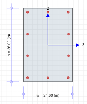
| Parameters | Column Designer | SAP 2000 v26 |
|---|---|---|
| Height (in) | 36 | |
| Width (in) | 24 | |
| fc’ (psi) | 4,000 | |
| fy (psi) | 40,000 | |
| Number of bars | 10 | |
| Corner Bars | #9 | |
| Bars along direction 2 and 3 | #8 | |
| Rebar Area (in2) | 8.71 | |
| Rebar Ratio | 1.01% | |
| Clear Cover (in) | 1.5 | |
SECTION PROPERTIES COMPARISON
| Properties | Units | Column Designer | SAP 2000 v26 | By hand |
|---|---|---|---|---|
| Basic Properties | ||||
| Area | in2 | 864.00 | 864.00 | 864.00 |
| Shear Area SA2 | in2 | 720.00 | 720.00 | 720.00 |
| Shear Area SA3 | in2 | 720.00 | 720.00 | 720.00 |
| Inertia, I22 | in4 | 41,472.00 | 41,472.00 | 41,472.00 |
| Inertia, I33 | in4 | 93,312.00 | 93,312.02 | 93,312.00 |
| Inertia, I32 | in4 | 0.00 | 0.00 | 0.00 |
| Section Bounds | ||||
| Total Width, Wtotal | in | 24.0 | 24.0 | 24.00 |
| Total Height, Htotal | in | 36.0 | 36.0 | 36.00 |
| Centroid, Xo | in | 0.00 | 0.00 | 0.00 |
| Centroid, Yo | in | 0.00 | 0.00 | 0.00 |
| Centroid, x̄ | in | 12.00 | 12.00 | 12.00 |
| Centroid, ȳ | in | 18.00 | 18.00 | 18.00 |
| Additional Properties | ||||
| Radius of gyration, R2 | in | 6.93 | 6.93 | 6.93 |
| Radius of Gyration, R3 | in | 10.39 | 10.39 | 10.39 |
| Section Modulus, S2-Left | in3 | 3,456.01 | 3,456.00 | 3,456.00 |
| Section Modulus, S2-Right | in3 | 3,456.01 | 3,456.00 | 3,456.00 |
| Section Modulus, S3-Top | in3 | 5,184.01 | 5,184.00 | 5,184.00 |
| Section Modulus, S3-Bottom | in3 | 5,184.01 | 5,184.00 | 5,184.00 |
CALCULATIONS BY HAND
Basic Properties
Area, \(A = b \times d\) = \(24\ \times 36 = 864\ {in}^{2}\)
Shear Area, SA2 \(= \frac{5}{6}\ \times \ A = \ \frac{5}{6}\ \times \ 864 = 720\ {in}^{2}\)
Shear Area, SA3 \(= \frac{5}{6}\ \times \ A = \ \frac{5}{6}\ \times \ 864 = 720\ {in}^{2}\)
Inertia, I22 \(= \frac{h}{12}\ \times \ w^{3} = \ \frac{36}{12}\ \times \ 24^{3} = 41,472\ {in}^{4}\)
Inertia, I33 \(= \frac{w}{12}\ \times \ h^{3} = \ \frac{24}{12}\ \times \ 36^{3} = 93,312\ {in}^{4}\)
Inertia, I23 = I32 \(= \\)0
Section Bounds
Total Width, Wtotal \(= w = 24\ in\)
Total Height, Htotal \(= h = 36\ in\)
Centroid, Xo \(= 0\ in\)
Centroid, Yo \(= 0\ in\\)
Centroid, x̄ \(= \frac{w}{2} = \ \frac{24}{2} = 12\ in\)
Centroid, ȳ \(= \frac{h}{2} = \ \frac{36}{2} = 18\ in\)
Additional Properties
Radius of gyration, R2 \(= \sqrt{\frac{I_{22}}{A}} = \sqrt{\frac{41472}{864}} = 6.93\ in\)
Radius of Gyration, R3 \(= \sqrt{\frac{I_{33}}{A}} = \sqrt{\frac{93312}{864}} = 10.39\ in\)
Section Modulus, S2-Left \(= \frac{I_{22}}{x_{0}} = \ \frac{41472}{12} = 3,456\ {in}^{3}\)
Section Modulus, S2-Right \(= \frac{I_{22}}{{W_{total} - x}_{0}} = \ \frac{41472}{24 - 12} = 3,456\ {in}^{3}\)
Section Modulus, S3-Top \(= \frac{I_{33}}{{H_{total} - y}_{0}} = \ \frac{93312}{36 - 18} = 5,184\ {in}^{3}\)
Section Modulus, S3-Bottom \(= \frac{I_{33}}{y_{0}} = \ \frac{93312}{18} = 5,184\ {in}^{3}\)
Section Properties Example 002
Section Properties of a Circular Column
GEOMETRY AND PROPERTIES
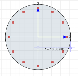
The section properties for a given circular section is tested in this example by comparing the results with SAP 2000 v26.
Note: Refer Section Properties Ex002.cdbx
The column section details and loading details are as tabulated below.
| Parameters | Column Designer | SAP 2000 v26 |
|---|---|---|
| Radius (in) | 18 | |
| fc’ (psi) | 4,000 | |
| fy (psi) | 40,000 | |
| Rebar | #9 | |
| Number of bars | 12 | |
| Rebar Area (in2) | 12.03 | |
| Rebar Ratio | 1.18% | |
| Clear Cover (in) | 1.5 | |
SECTION PROPERTIES COMPARISON
| Properties | Units | Column Designer | SAP 2000 v26 | By Hand |
|---|---|---|---|---|
| Basic Properties | ||||
| Area | in2 | 1017.88 | 1011.35 | 1,017.88 |
| Shear Area SA2 | in2 | 916.09 | 913.01 | 916.09 |
| Shear Area SA3 | in2 | 916.09 | 913.01 | 916.09 |
| Inertia, I22 | in4 | 82,447.96 | 81,395.00 | 82,447.96 |
| Inertia, I33 | in4 | 82,447.96 | 81,395.00 | 82,447.96 |
| Inertia, I32 | in4 | 0.00 | 0.00 | 0.00 |
| Section Bounds | ||||
| Total Width, Wtotal | in | 36.00 | 36.00 | 36.00 |
| Total Height, Htotal | in | 36.00 | 36.00 | 36.00 |
| Centroid, Xo | in | 0.00 | 0.00 | 0.00 |
| Centroid, Yo | in | 0.00 | 0.00 | 0.00 |
| Centroid, x | in | 18.00 | 18.00 | 18.00 |
| Centroid, y | in | 18.00 | 18.00 | 18.00 |
| Additional Properties | ||||
| Radius of gyration, R2 | in | 9.00 | 8.97 | 9.00 |
| Radius of Gyration, R3 | in | 9.00 | 8.97 | 9.00 |
| Section Modulus, S2-Left | in3 | 4,580.45 | 4,521.92 | 4,580.44 |
| Section Modulus, S2-Right | in3 | 4,580.45 | 4,521.92 | 4,580.44 |
| Section Modulus, S3-Top | in3 | 4,580.45 | 4,521.92 | 4,580.44 |
| Section Modulus, S3-Bottom | in3 | 4,580.45 | 4,521.92 | 4,580.44 |
CALCULATIONS BY HAND
Basic Properties
Area, \(A = \pi \times r^{2}\) = \(\pi\ \times \ 18^{2} = 1,017.88\ {in}^{2}\)
Shear Area, SA2 \(= \frac{5}{6}\ \times \ A = \ \frac{5}{6}\ \times \ 656692.18 = 916.09\ {in}^{2}\)
Shear Area, SA3 \(= \frac{5}{6}\ \times \ A = \ \frac{5}{6}\ \times \ 656692.18 = 916.09\ {in}^{2}\)
Inertia, I22 \(= \frac{\pi \times r^{4}}{4}\ = \ \frac{\pi \times 18^{4}}{4} = 82,447.96\ {in}^{4}\)
Inertia, I33 \(= \frac{\pi \times r^{4}}{4}\ = \ \frac{\pi \times 18^{4}}{4} = 82,447.96\ {in}^{4}\)
Inertia, I23 = I32 \(= \\)0 \({in}^{4}\)
Section Bounds
Total Width, Wtotal \(= r \times 2 = 36\ in\)
Total Height, Htotal \(= r \times 2 = 36\ in\)
Centroid, Xo \(= r = 18\ in\)
Centroid, Yo \(= r = 18\ in\\)
Centroid, x̄ \(= \frac{w}{2} = \ \frac{24}{2} = 12\ in\)
Centroid, ȳ \(= \frac{h}{2} = \ \frac{36}{2} = 18\ in\)
Additional Properties
Radius of gyration, R2 \(= \sqrt{\frac{I_{22}}{A}} = \sqrt{\frac{82447.96}{1017.88}} = 9\ in\)
Radius of Gyration, R3 \(= \sqrt{\frac{I_{33}}{A}} = \sqrt{\frac{82447.96}{1017.88}} = 9\ in\)
Section Modulus, S2-Left \(= \frac{I_{22}}{x_{0}} = \ \frac{82447.96}{18} = 4,580.44\ {in}^{3}\)
Section Modulus, S2-Right \(= \frac{I_{22}}{{W_{total} - x}_{0}} = \ \frac{82447.96}{36 - 18} = 4,580.44\ {in}^{3}\)
Section Modulus, S3-Top \(= \frac{I_{33}}{{H_{total} - y}_{0}} = \ \frac{82447.96}{36 - 18} = 4,580.44\ {in}^{3}\)
Section Modulus, S3-Bottom \(= \frac{I_{33}}{y_{0}} = \ \frac{82447.96}{18} = 4,580.44\ {in}^{3}\)
Section Properties Example 003
Section Properties of a T-Section
GEOMETRY AND PROPERTIES
The section properties for a given T-section is tested in this example by comparing the results with SAP 2000 v26.
Note: Refer Section Properties Ex003.cdbx
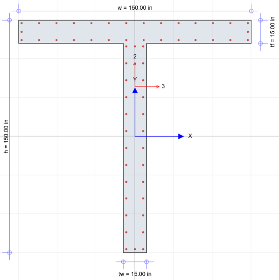 The column section details and loading details are as tabulated below.
| Parameters | Column Designer | SAP 2000 v26 |
|---|---|---|
| Height (in) | 150 | |
| Width (in) | 150 | |
| Web Width (in) | 15 | |
| Flange Height (in) | 15 | |
| fc’ (psi) | 6,000 | |
| fy (psi) | 60,000 | |
| Number of bars | 58 | |
| Corner Bars | #8 | |
| Bars along direction 2 and 3 | #8 | |
| Rebar Area (in2) | 45.55 | |
| Rebar Ratio | 1.07% | |
| Clear Cover (in) | 1.5 | |
SECTION PROPERTIES COMPARISON
| Properties | Units | Column Designer | SAP 2000 v26 | By hand |
|---|---|---|---|---|
| Basic Properties | ||||
| Area | in2 | 4,275.00 | 4,275.00 | 4,275.00 |
| Shear Area SA2 | in2 | 2,012.75 | 2,006.05 | - |
| Shear Area SA3 | in2 | 2,259.24 | 2,298.55 | - |
| Inertia, I22 | in4 | 4,256,681.00 | 4,256,719.00 | 4,256,718.75 |
| Inertia, I33 | in4 | 9,122,700.93 | 9,112,722.00 | 9,112,722.04 |
| Inertia, I32 | in4 | 0.00 | 0.00 | 0.00 |
| Section Bounds | ||||
| Total Width, Wtotal | in | 150.00 | 150.00 | 150.00 |
| Total Height, Htotal | in | 150.00 | 150.00 | 150.00 |
| Centroid, Xo | in | 0.00 | 0.00 | 0.00 |
| Centroid, Yo | in | 31.97 | 31.97 | 31.97 |
| Centroid, x̄ | in | 75.00 | 75.00 | 75.00 |
| Centroid, ȳ | in | 106.97 | 106.97 | 106.97 |
| Additional Properties | ||||
| Radius of Gyration, R2 | in | 31.55 | 31.55 | 31.56 |
| Radius of Gyration, R3 | in | 46.17 | 46.17 | 46.17 |
| Section Modulus, S2-Left | in3 | 56,755.80 | 56,756.00 | 56,756.25 |
| Section Modulus, S2-Right | in3 | 56,755.80 | 56,756.00 | 56,756.25 |
| Section Modulus, S3-Top | in3 | 211,794.14 | 211,794.00 | 211,794.15 |
| Section Modulus, S3-Bottom | in3 | 85,186.50 | 85,187.00 | 85,186.58 |
CALCULATIONS BY HAND
Basic Properties
Area, \(A = A_{1} + A_{2} = 2,025 + 2,250 = 4,275\ {in}^{2}\)
- \(A_{1} = \left( h - t_{f} \right) \times t_{w}\)
\(= (150 - 15) \times 150\)
\(= 2,025\ {in}^{2}\)
- \(A_{2} = w \times t_{f}\)
\(= 150 \times 15\)
\(= 2,250\ {in}^{2}\)
Inertia, \(I22 = I22_{a} + I22_{b} = 37,968.75 + 4,218,750 = 4,256,718.75\ {in}^{4}\)
- \(I22_{a} = \frac{\left( h - t_{f} \right) \times {t_{w}}^{3}\ }{12} + A_{1} \times \left( x_{0} - x_{1} \right)^{2}\)
\(= \frac{(150 - 15) \times 150^{3}\ }{12} + 2,025 \times (75 - 75)^{2}\)
\(= 37,968.75\ {in}^{4}\)
- \(I22_{b} = \frac{t_{f} \times w^{3}\ }{12} + A_{2} \times \left( x_{0} - x_{2} \right)^{2}\)
\(= \frac{15 \times 150^{3}\ }{12} + 2,250 \times (75 - 75)^{2}\)
\(= 4,218,750\ {in}^{4}\)
Inertia, \(I33 = I33_{a} + I33_{b} = 6,230,766.53 + 2,881,955.51 = 9,112,722.04\ {in}^{4}\)
- \(I33_{a} = \frac{t_{w} \times \left( h - t_{f} \right)^{3}\ }{12} + A_{1} \times \left( y_{0} - y_{1} \right)^{2}\)
\(= \frac{15 \times (150 - 15)^{3}\ }{12} + 2,025 \times (106.97 - 67.5)^{2}\)
\(= 6,230,766.53\ {in}^{4}\)
- \(I33_{b} = \frac{w \times {t_{f}}^{3}\ }{12} + A_{2} \times \left( x_{0} - x_{2} \right)^{2}\)
\(= \frac{150 \times 15^{3}\ }{12} + 2,250 \times (106.97 - 142.5)^{2}\)
\(= 2,881,955.51\ {in}^{4}\)
- Inertia, I23 = I32 \(= \\)0
Section Bounds
Total Width, Wtotal \(= w = 150\ in\)
Total Height, Htotal \(= h = 150\ in\)
Centroid, Xo \(= 0\ in\)
Centroid, Yo \(= 31.97\ in\\)
Centroid, x̄ \(= 75.00\ in\)
Centroid, ȳ \(= 106.97\ in\\)
Additional Properties
Radius of gyration, R2 \(= \sqrt{\frac{I_{22}}{A}} = \sqrt{\frac{4,256,718.75}{4,275.00}} = 31.56\ in\)
Radius of Gyration, R3 \(= \sqrt{\frac{I_{33}}{A}} = \sqrt{\frac{9,112,722.04}{4,275.00}} = 46.17\ in\)
Section Modulus, S2-Left \(= \frac{I_{22}}{x_{0}} = \ \frac{4,256,718.75}{75.00} = 56,756.25\ {in}^{3}\)
Section Modulus, S2-Right \(= \frac{I_{22}}{{W_{total} - x}_{0}} = \ \frac{4,256,718.75}{150 - 75} = 56,756.25\ {in}^{3}\)
Section Modulus, S3-Top \(= \frac{I_{33}}{{H_{total} - y}_{0}} = \ \frac{9,112,722.04}{150 - 106.97} = 211,794.15\ {in}^{3}\)
Section Modulus, S3-Bottom \(= \frac{I_{33}}{y_{0}} = \ \frac{9,112,722.04}{106.97} = 85,186.58\ {in}^{3}\)
P-M Interaction
ACI 318-19 PM Example 001
P-M Interaction Check for Rectangular Column
GEOMETRY AND PROPERTIES
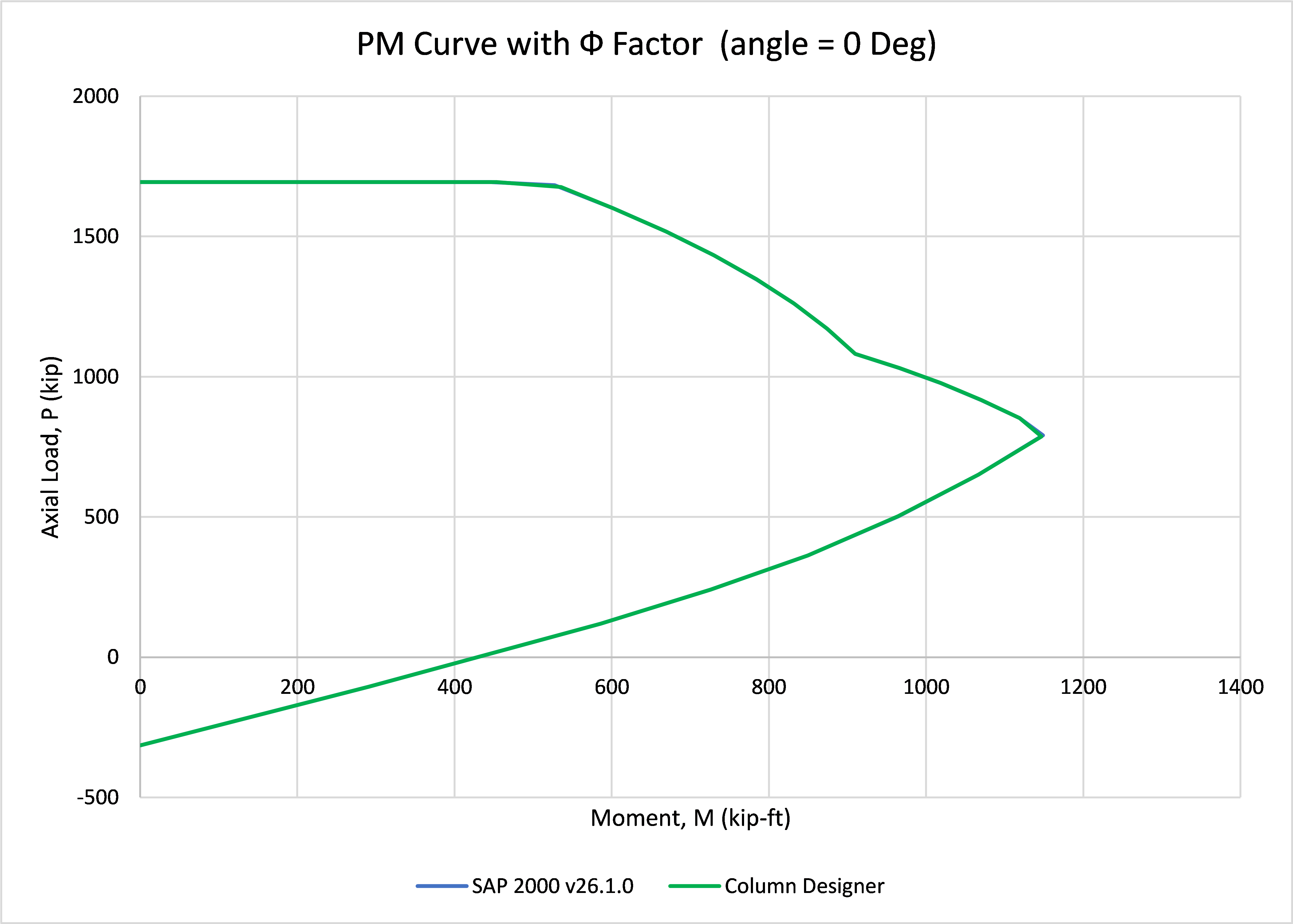
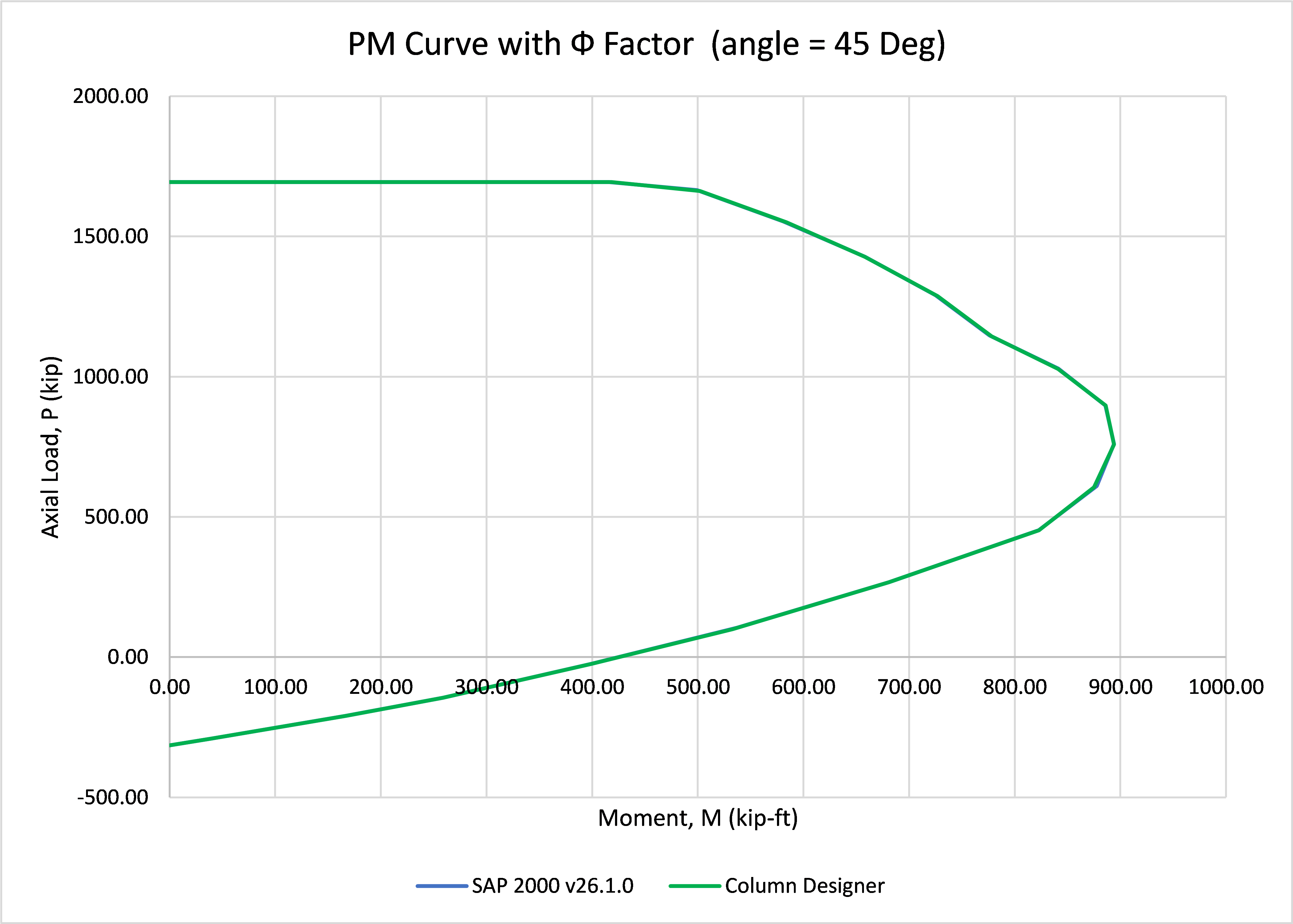
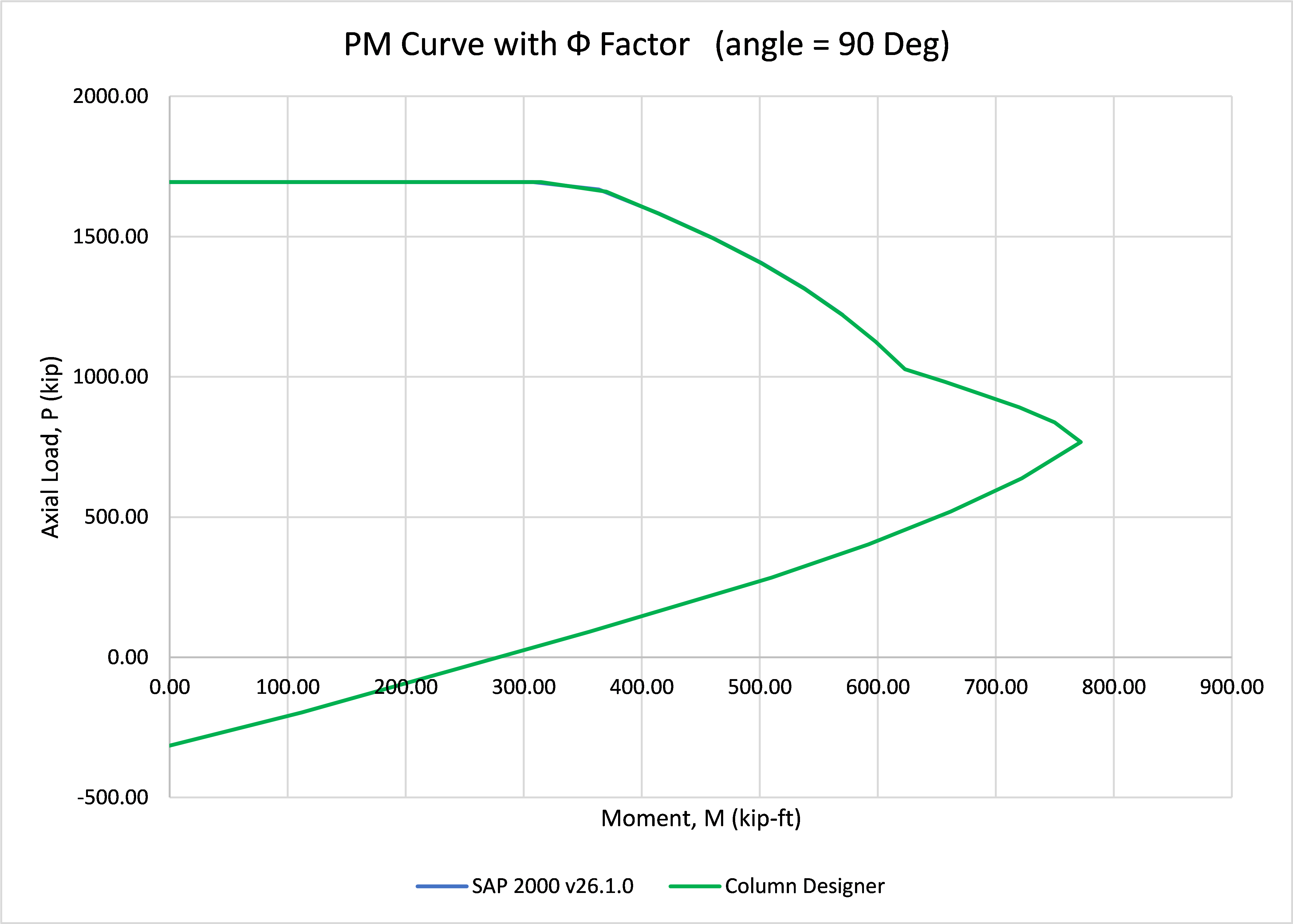
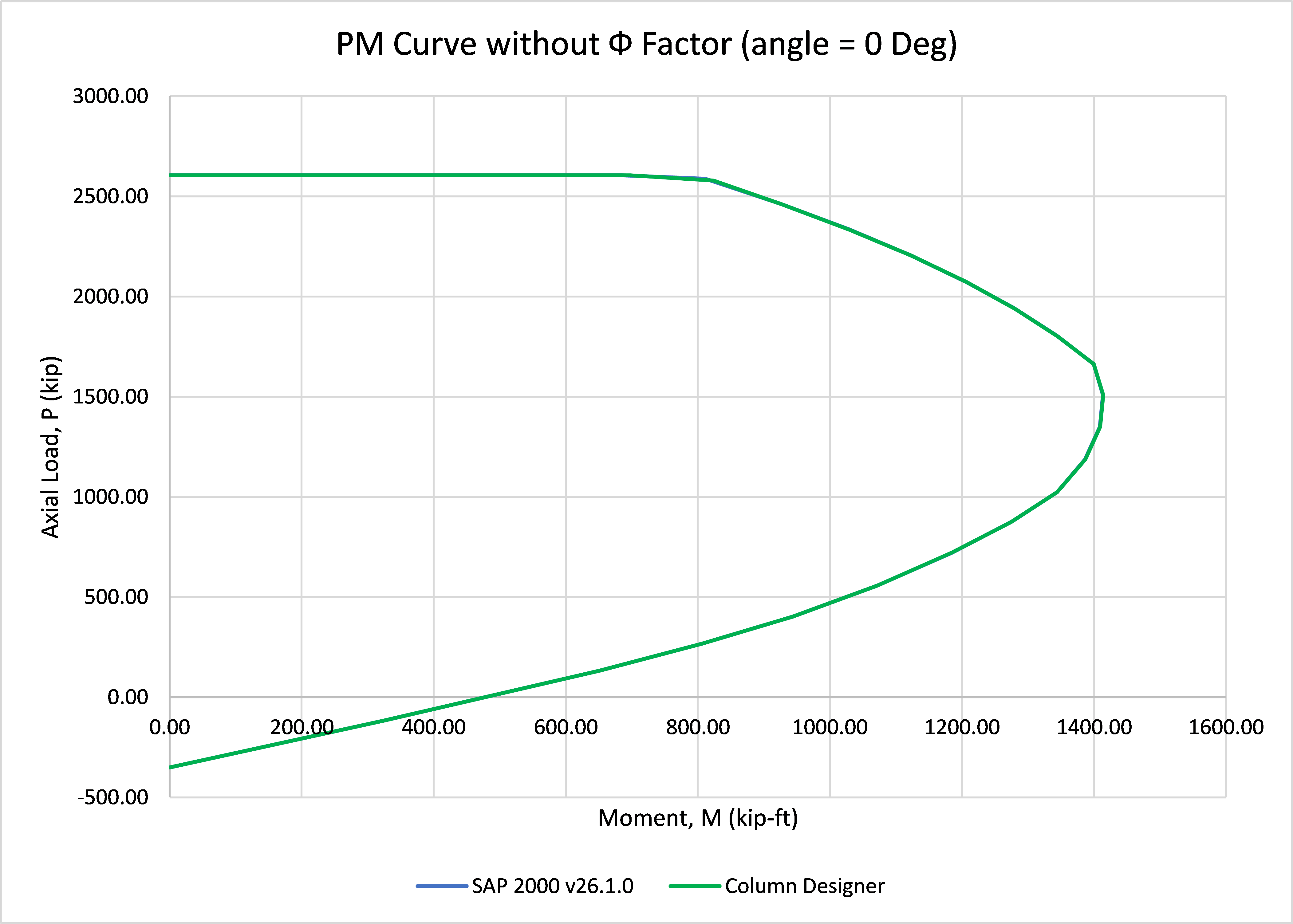
The P-M Interaction Check for a given rectangular section is tested in this example by comparing the P-M results with SAP 2000 v26.
Note: Refer PM Ex001.cdbx
The column section details are as tabulated below.
| Parameters | Column Designer | SAP 2000 v26 |
|---|---|---|
| Code | ACI 318-19 | |
| Height (in) | 36 | |
| Width (in) | 24 | |
| fc’ (psi) | 4,000 | |
| fy (psi) | 40,000 | |
| Number of bars | 10 | |
| Corner Bars | #9 | |
| Bars along direction 2 and 3 | #8 | |
| Rebar Area (in2) | 8.71 | |
| Rebar Ratio | 1.01% | |
| Clear Cover (in) | 1.5 | |
P-M INTERACTION COMPARISON WITH Ф FACTOR
P-M INTERACTION COMPARISON WITHOUT Ф FACTOR
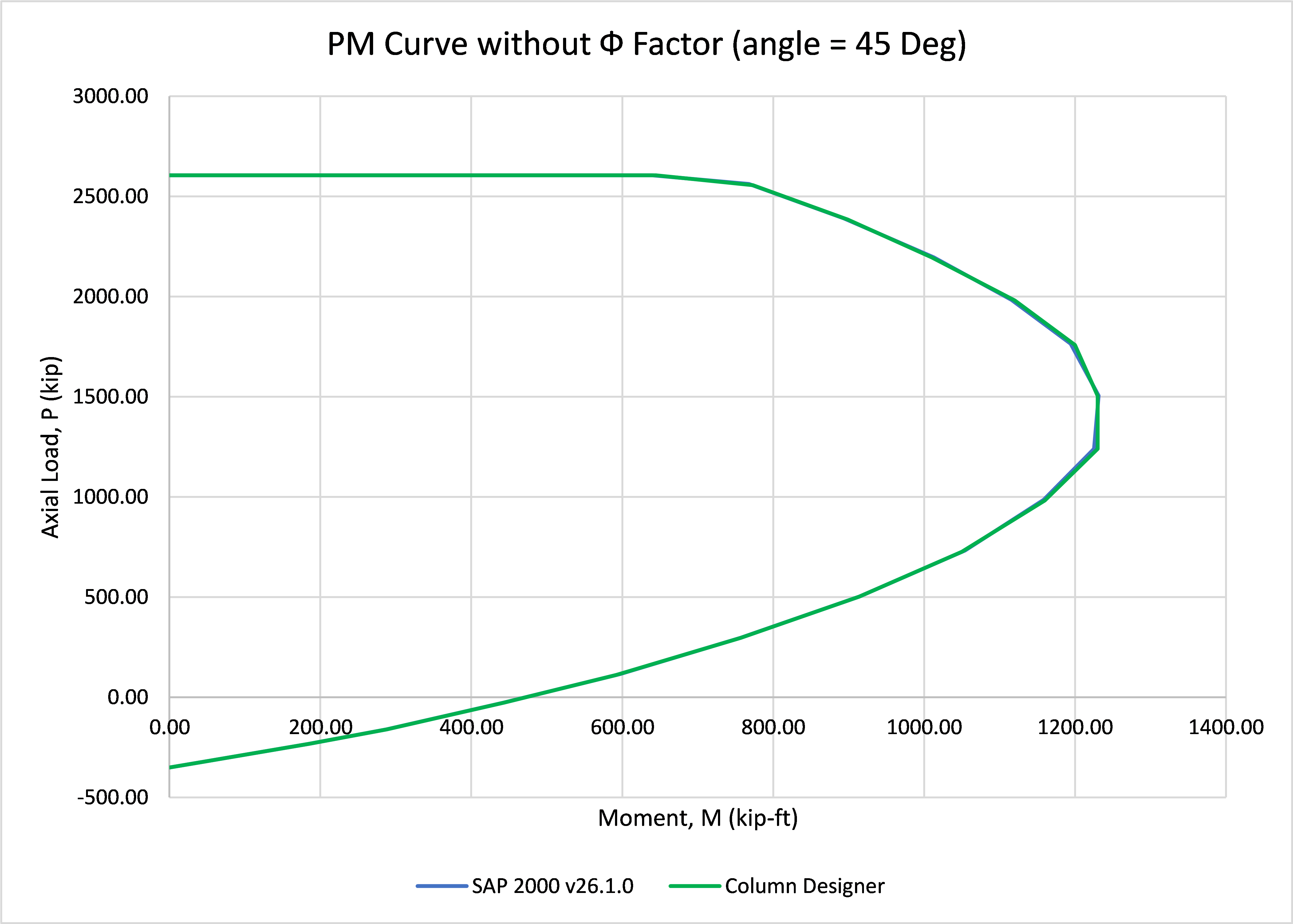
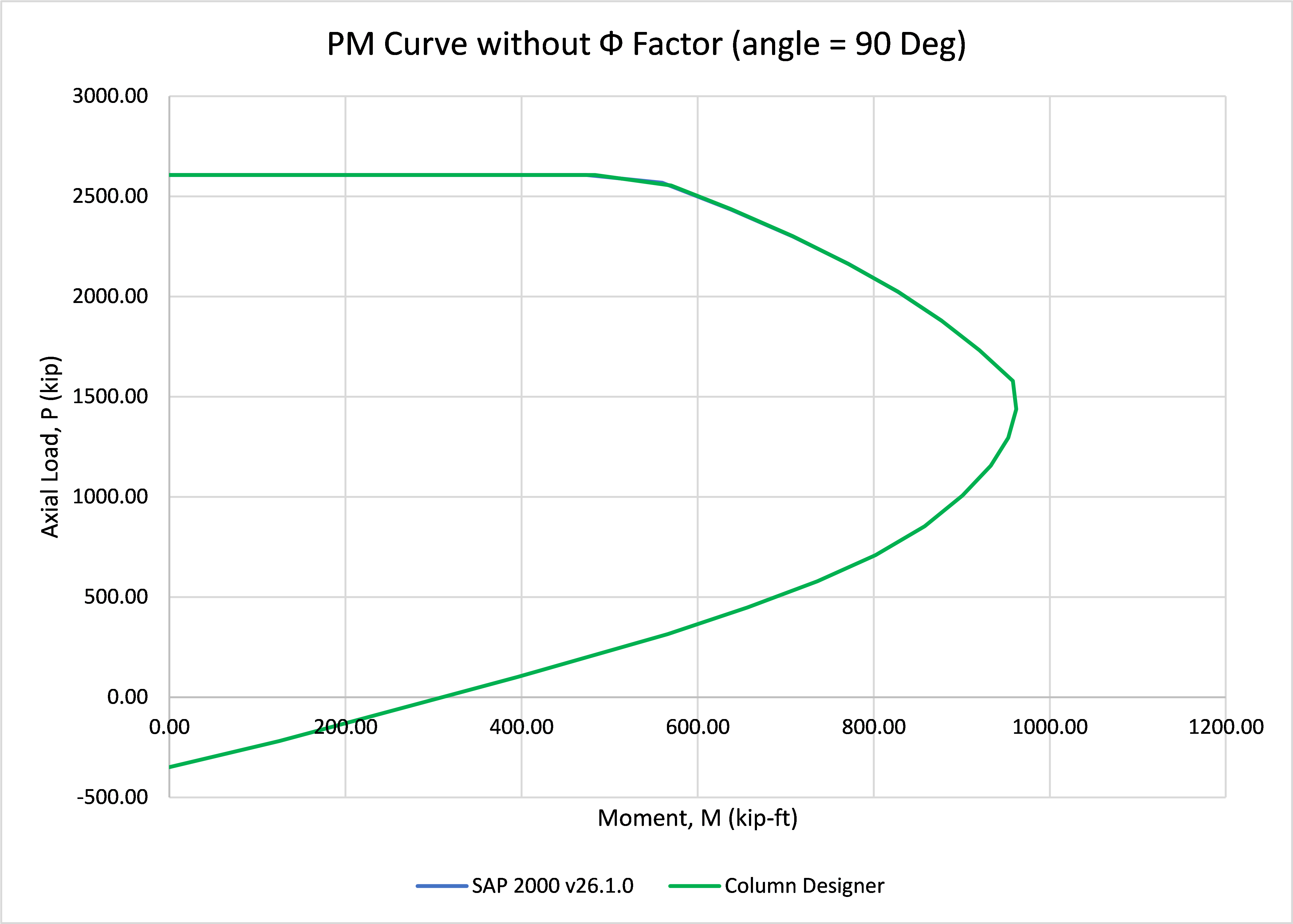
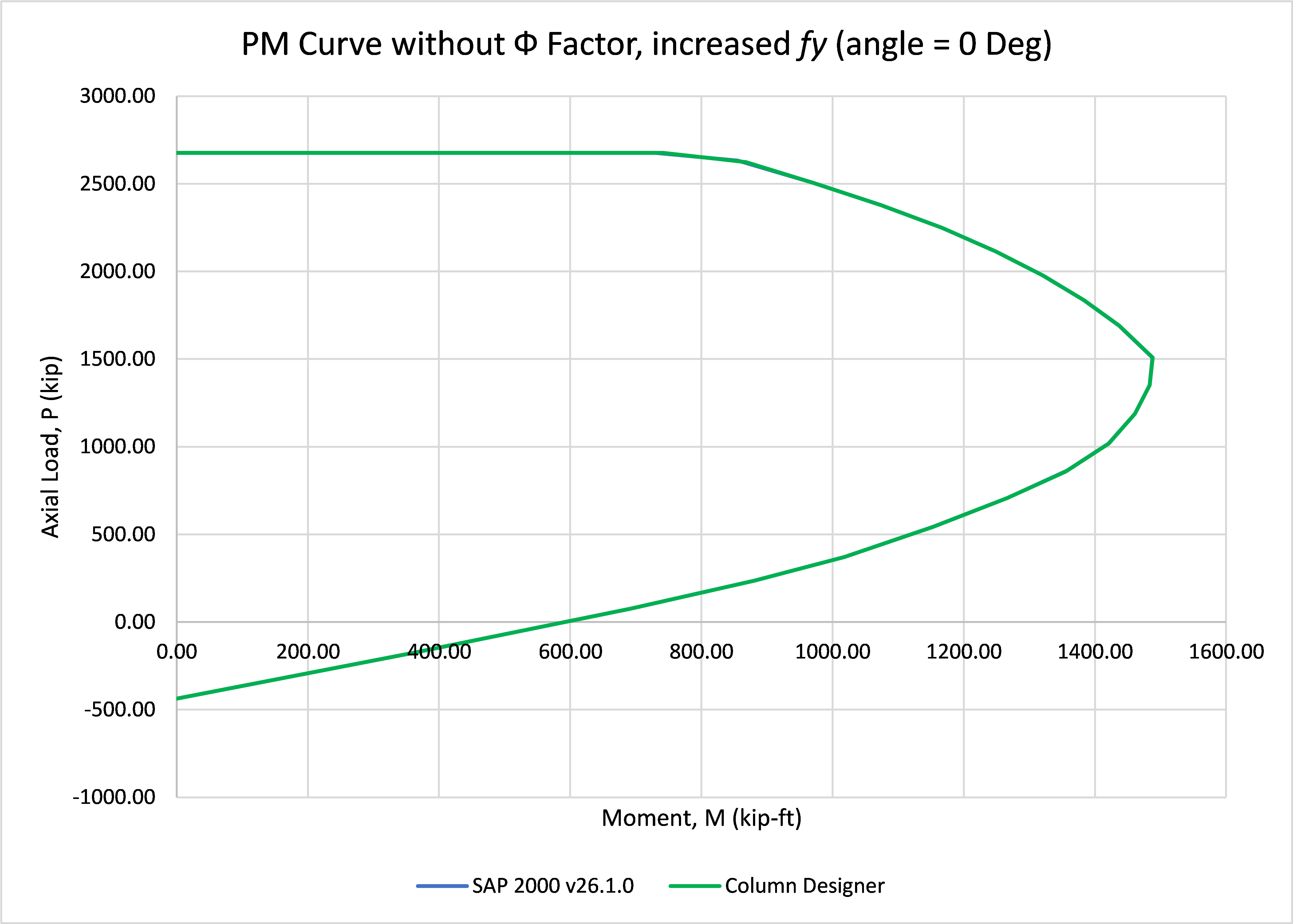
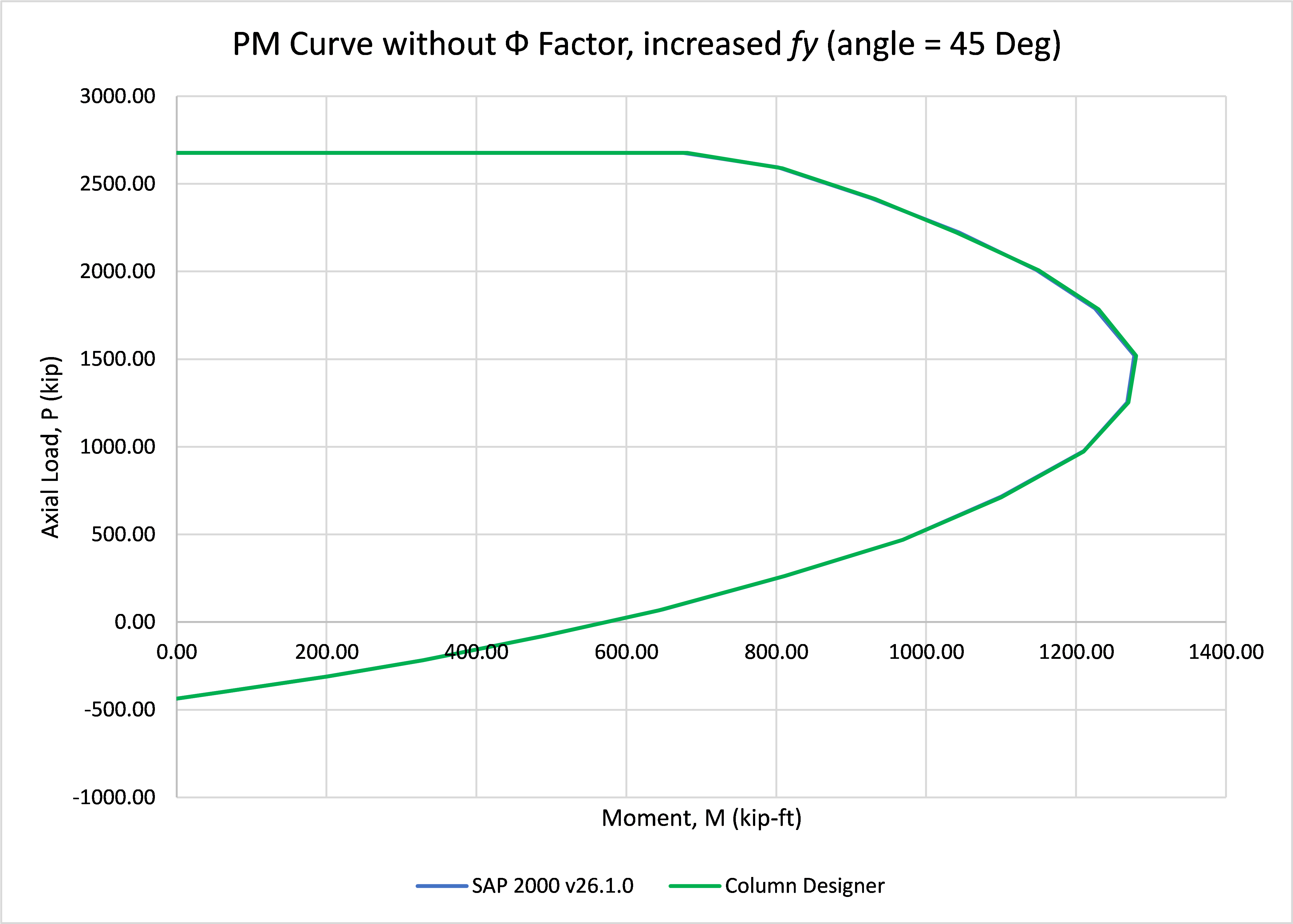
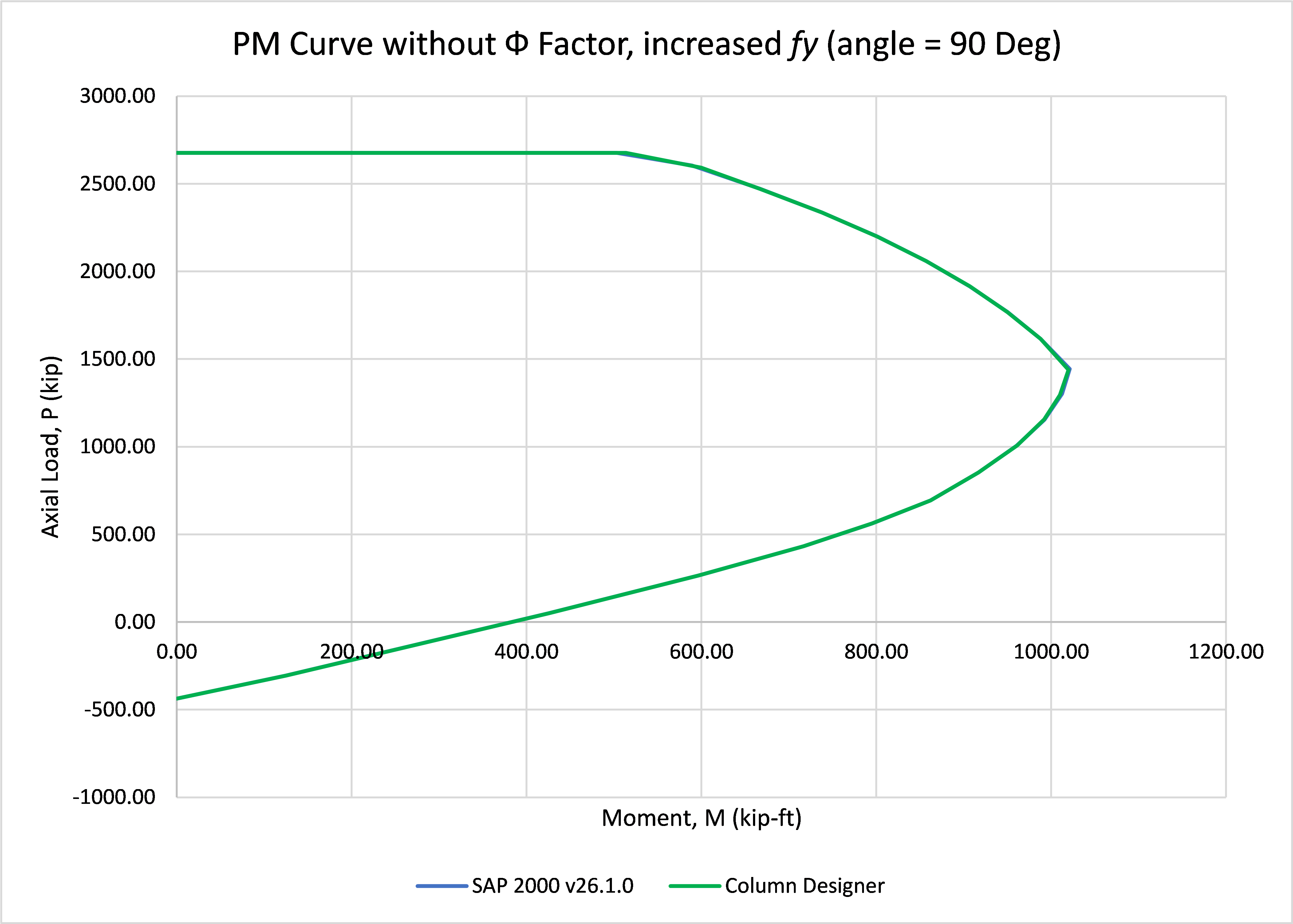
P-M INTERACTION COMPARISON WITHOUT Ф FACTOR AND INCREASED FY
ACI 318-19 PM Example 002
P-M Interaction Check for Circular Column
GEOMETRY AND PROPERTIES
The P-M Interaction Check for a given circular section is tested in this example by comparing the results with SAP 2000 v26.
Note: Refer PM Ex002.cdbx
The column section details are as tabulated below.
| Parameters | Column Designer v12 | SAP 2000 v26 |
|---|---|---|
| ACI Code | ACI 318-19 | |
| Radius (in) | 18 | |
| fc’ (psi) | 4,000 | |
| fy (psi) | 40,000 | |
| Rebar | #9 | |
| Number of bars | 12 | |
| Rebar Area (in2) | 12.03 | |
| Rebar Ratio | 1.18% | |
| Clear Cover (in) | 1.5 | |
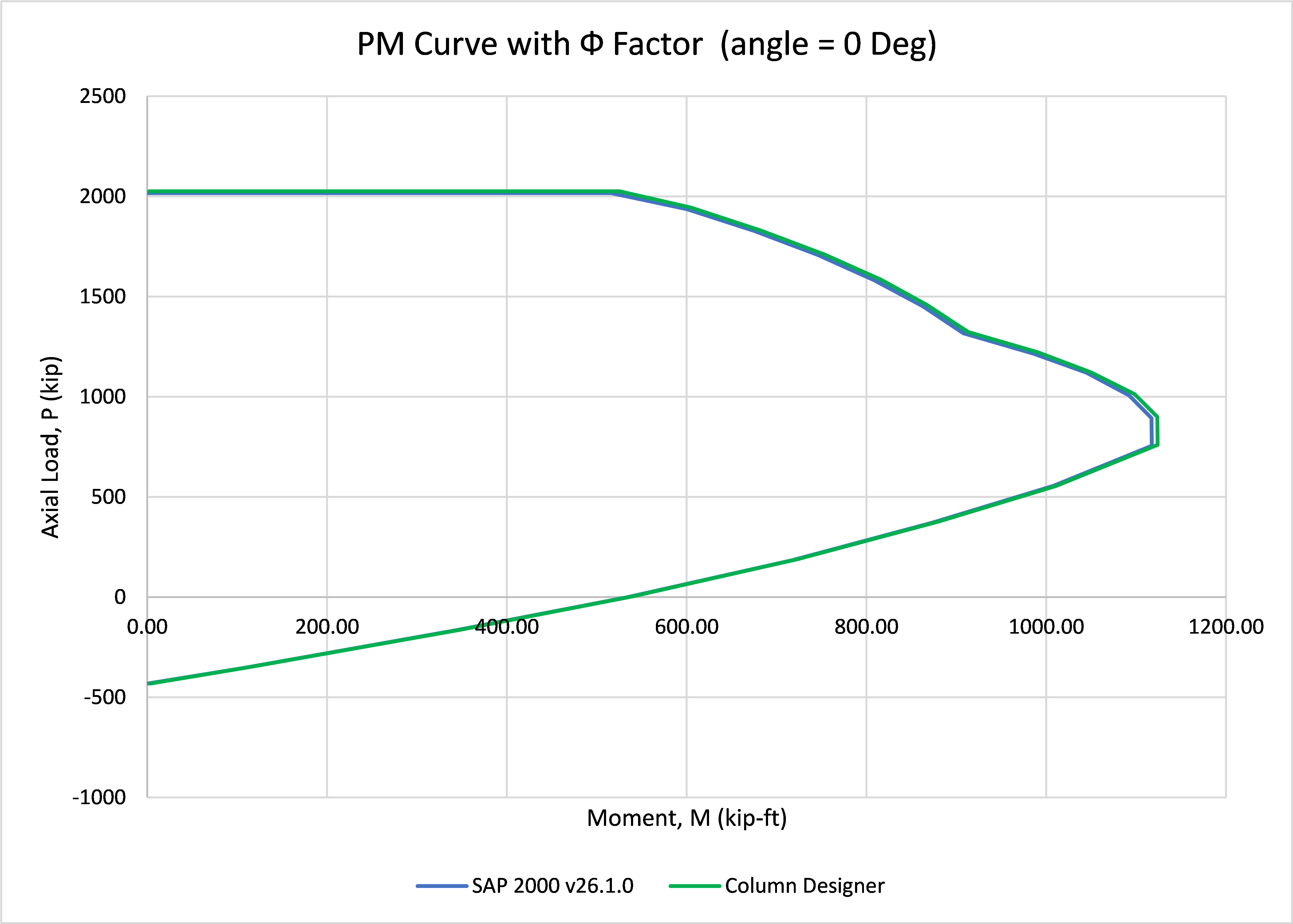
P-M INTERACTION COMPARISON WITH Ф FACTOR
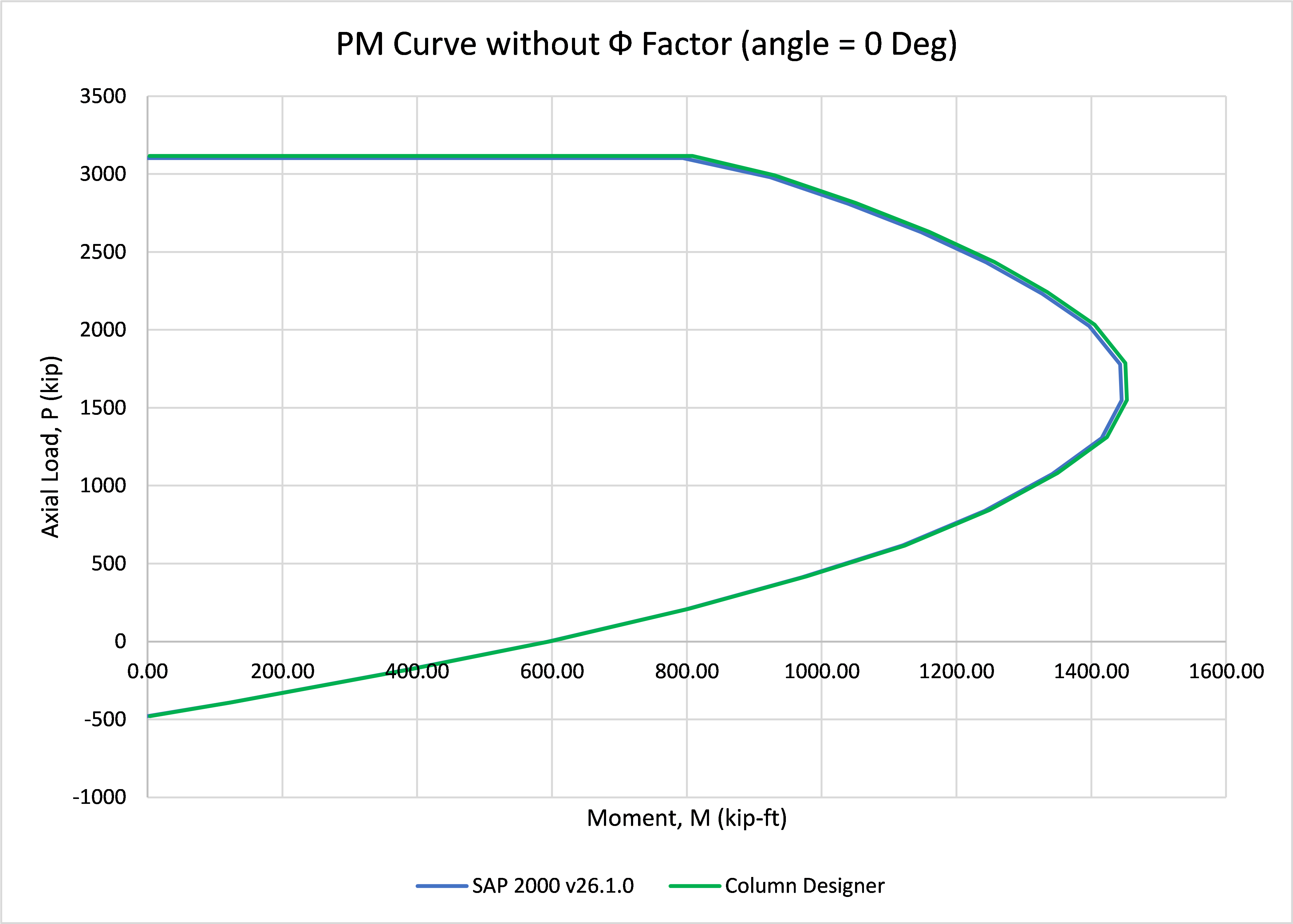
P-M INTERACTION COMPARISON WITHOUT Ф FACTOR
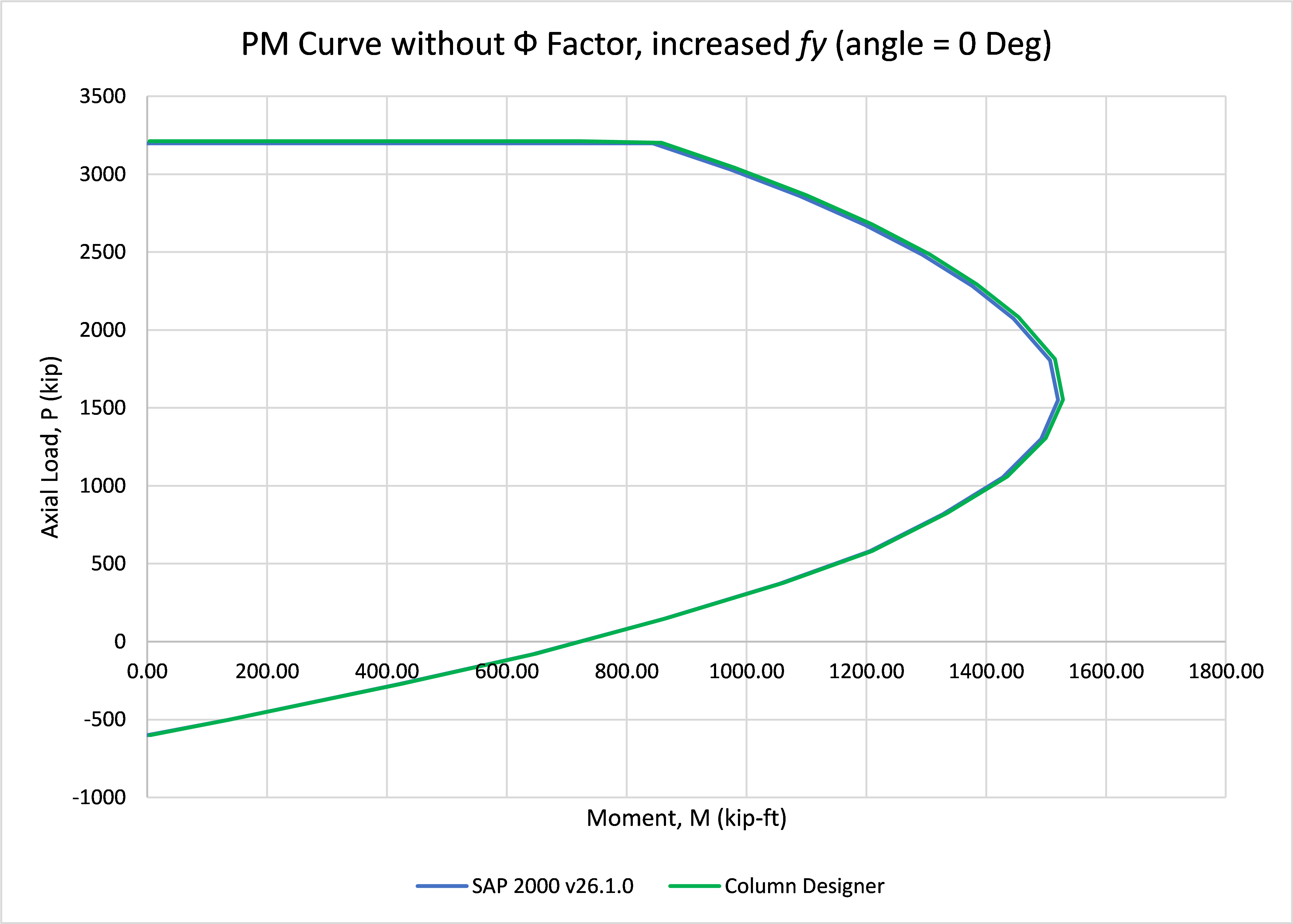
P-M INTERACTION COMPARISON WITHOUT Ф INCREASED FY
ACI 318-19 PM Example 003
P-M Interaction Check for T-Section
GEOMETRY AND PROPERTIES
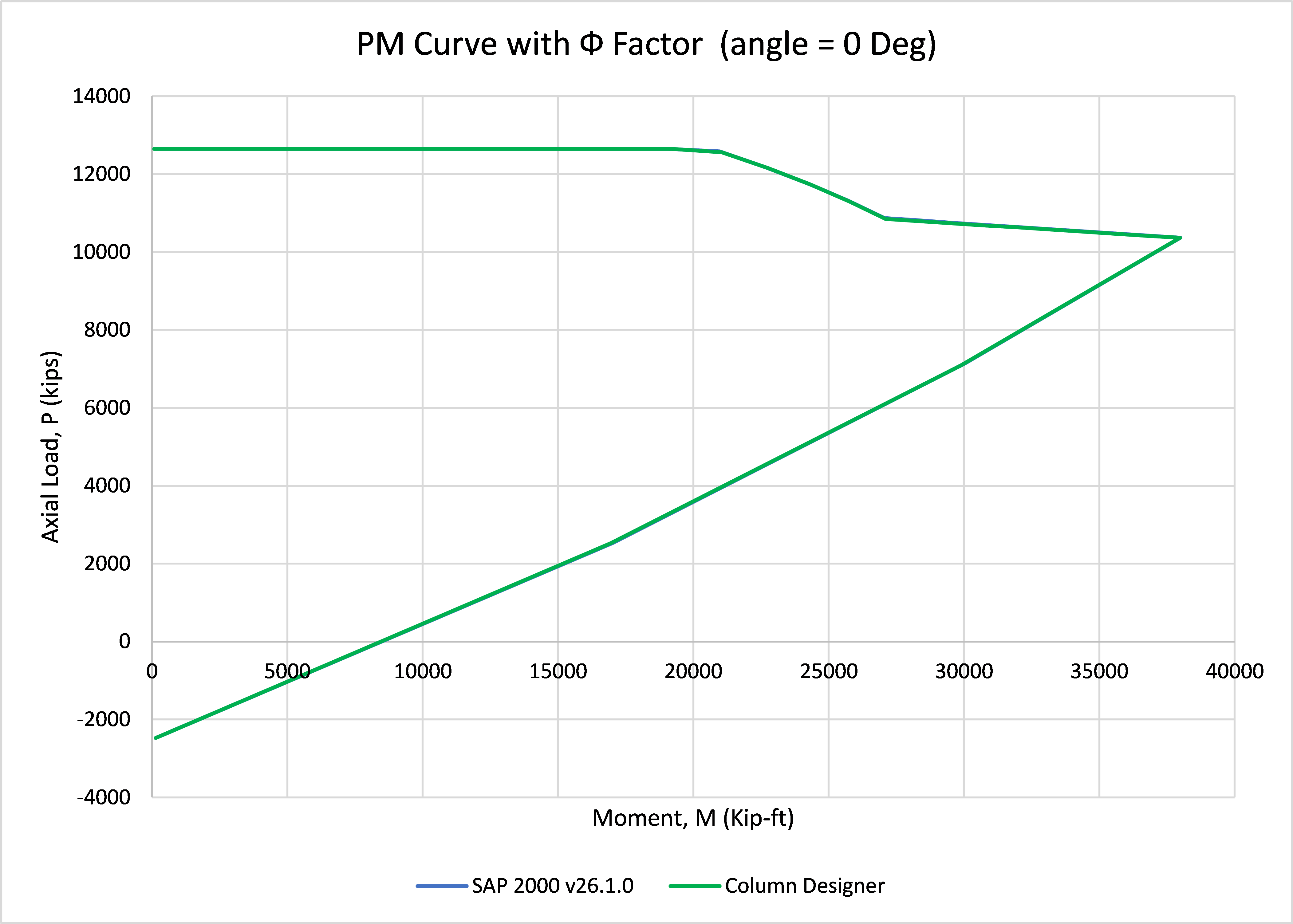
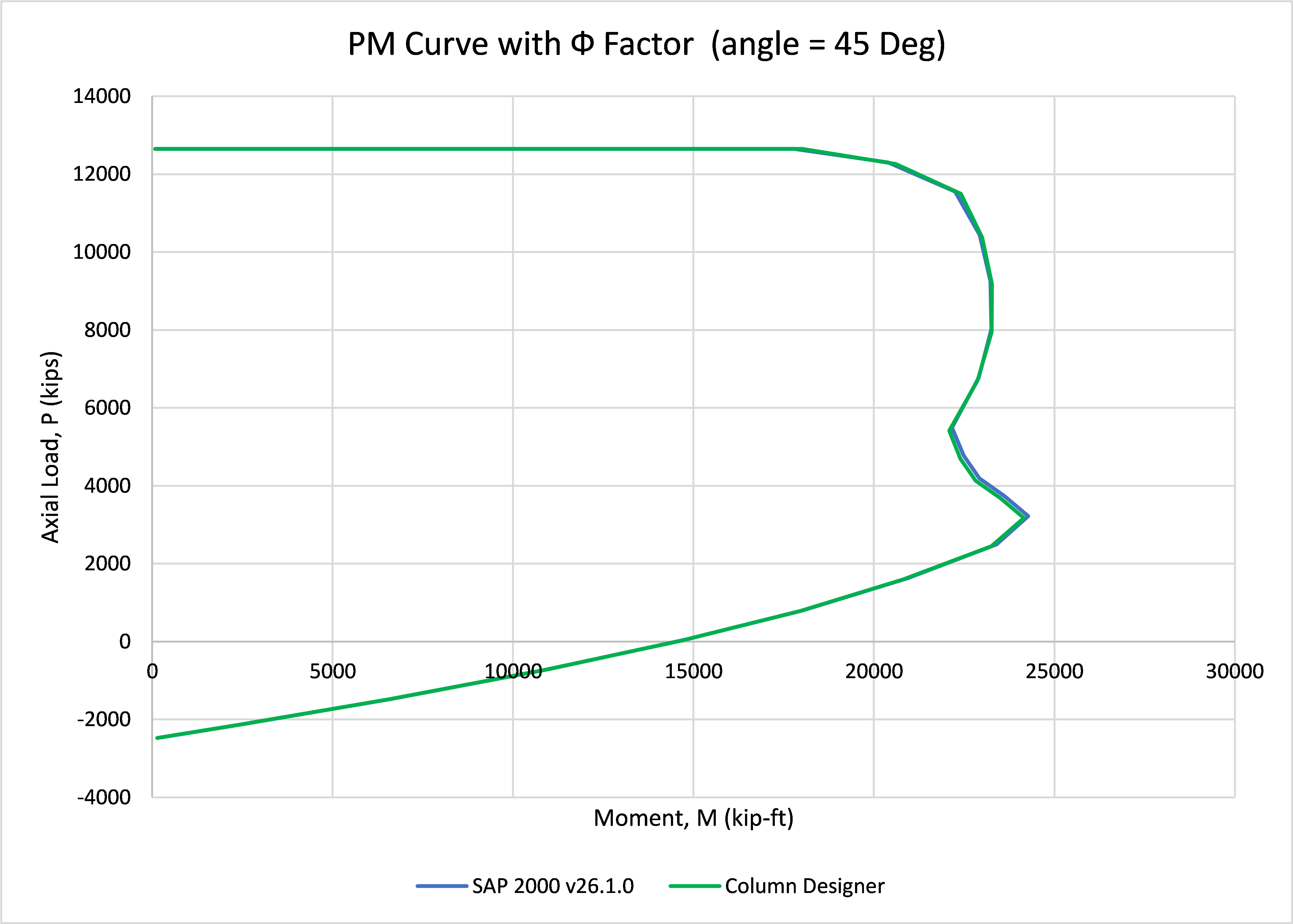
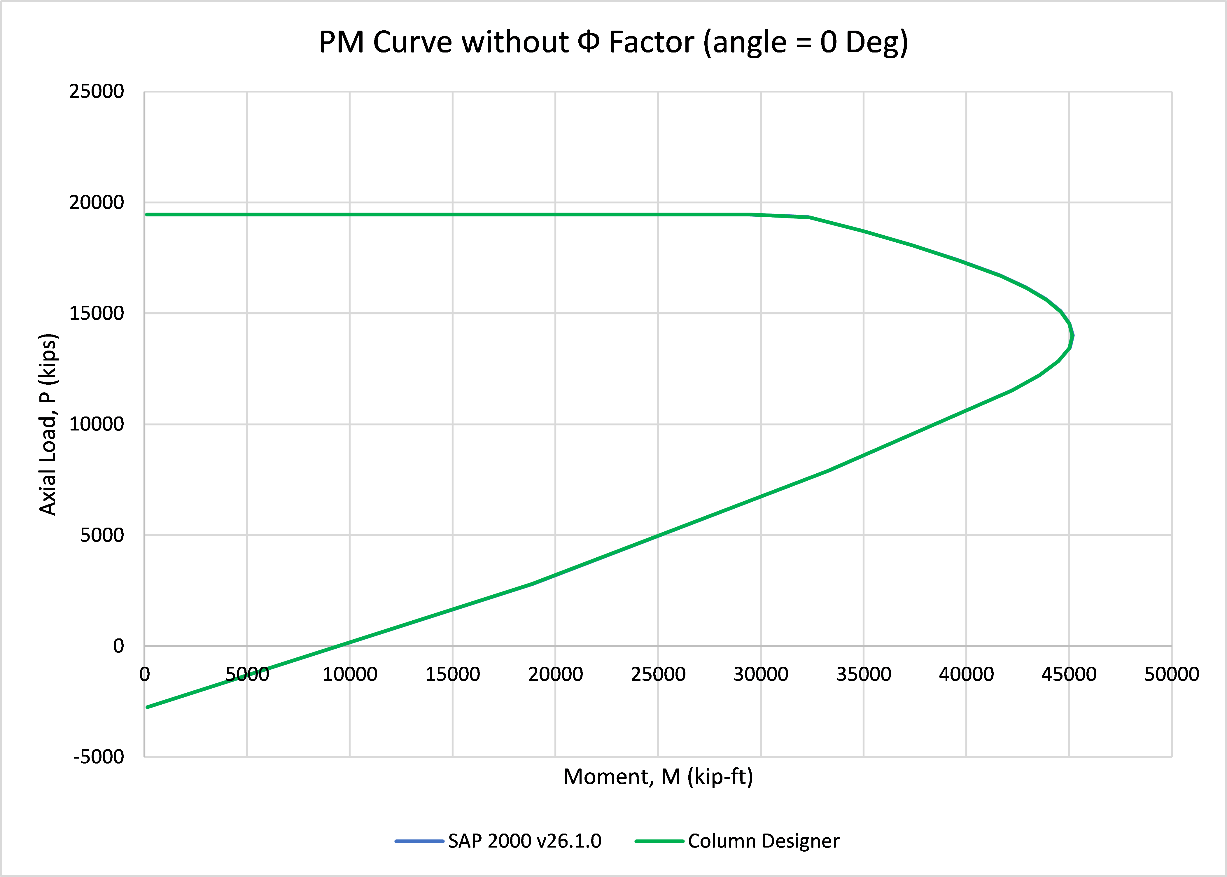
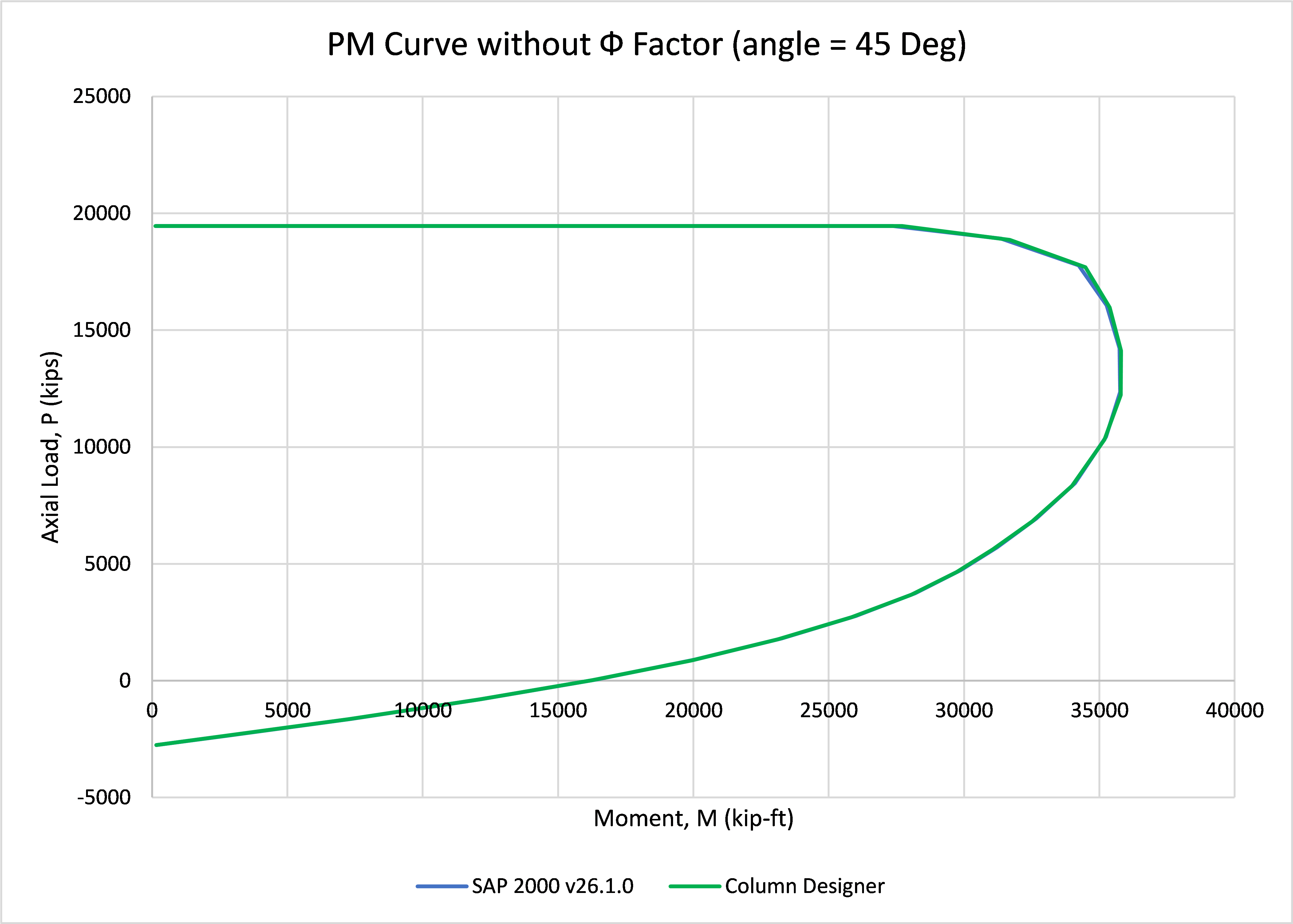
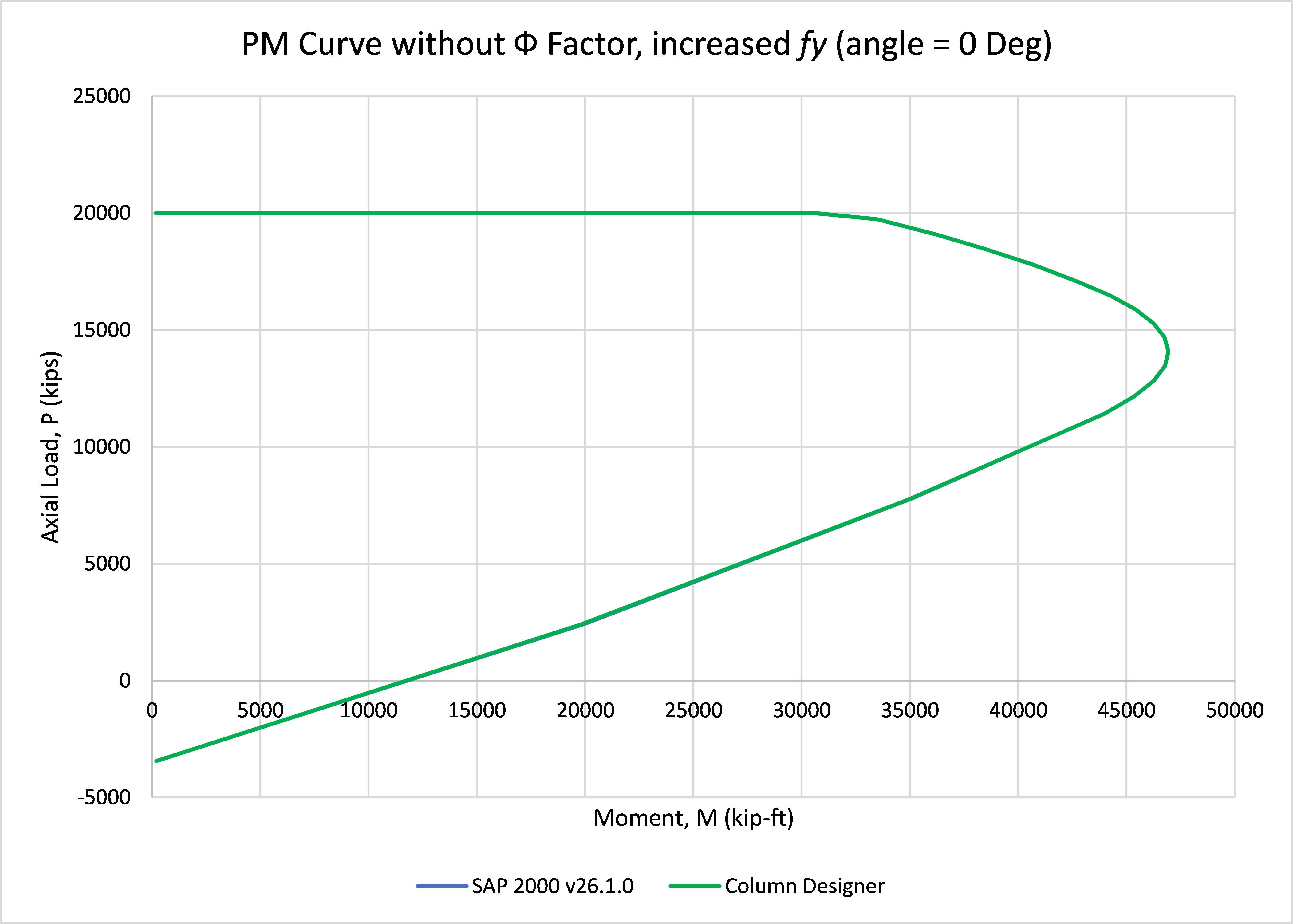
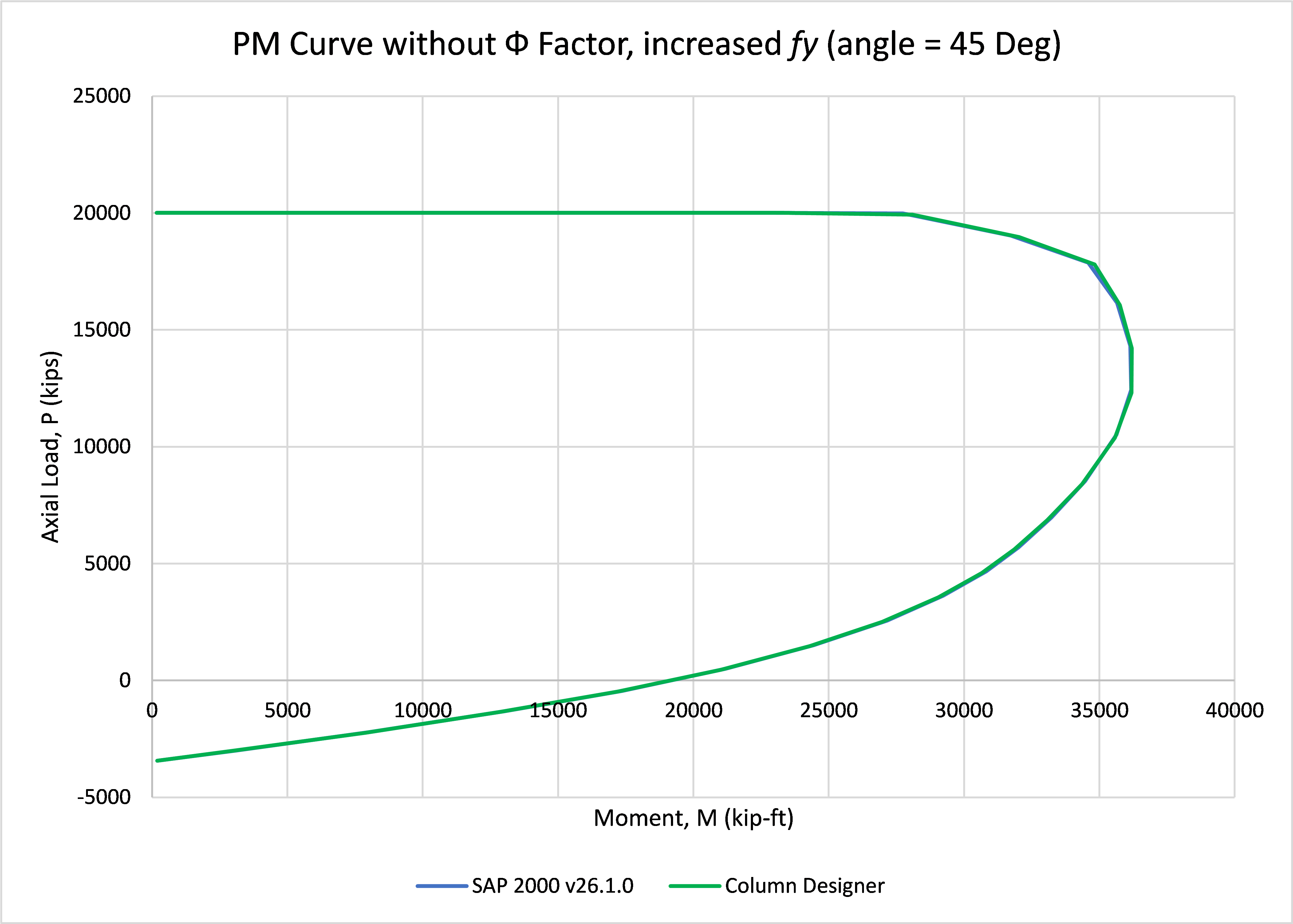
The P-M Interaction Check for a given T-section is tested in this example by comparing the P-M results with SAP 2000 v26.
Note: Refer PM Ex003.cdbx
The column section details are as tabulated below.
| Parameters | Column Designer | SAP 2000 v26 |
|---|---|---|
| Code | ACI 318-19 | |
| Height (in) | 150 | |
| Width (in) | 150 | |
| Web Width (in) | 15 | |
| Flange Height (in) | 15 | |
| fc’ (psi) | 6,000 | |
| fy (psi) | 60,000 | |
| Number of bars | 58 | |
| Corner Bars | #8 | |
| Bars along direction 2 and 3 | #8 | |
| Rebar Area (in2) | 45.55 | |
| Rebar Ratio | 1.07% | |
| Clear Cover (in) | 1.5 | |
P-M INTERACTION COMPARISON WITH Ф FACTOR
P-M INTERACTION COMPARISON WITHOUT Ф FACTOR
P-M INTERACTION COMPARISON WITHOUT Ф FACTOR AND INCREASED FY
ACI 318-19 PM Example 004
P-M Interaction Check for Inverted T-Section
GEOMETRY AND PROPERTIES
The P-M Interaction Check for a given Inverted T-section is tested in this example by comparing the P-M results with SAP 2000 v26.
Note: Refer PM Ex004.cdbx
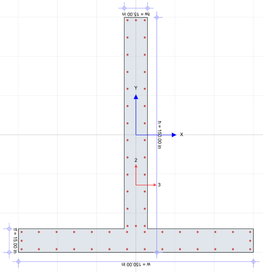 The column section details are as tabulated below.
| Parameters | Column Designer | SAP 2000 v26 |
|---|---|---|
| Code | ACI 318-19 | |
| Height (in) | 150 | |
| Width (in) | 150 | |
| Web Width (in) | 15 | |
| Flange Height (in) | 15 | |
| fc’ (psi) | 6,000 | |
| fy (psi) | 60,000 | |
| Number of bars | 58 | |
| Corner Bars | #8 | |
| Bars along direction 2 and 3 | #8 | |
| Rebar Area (in2) | 45.55 | |
| Rebar Ratio | 1.07% | |
| Clear Cover (in) | 1.5 | |
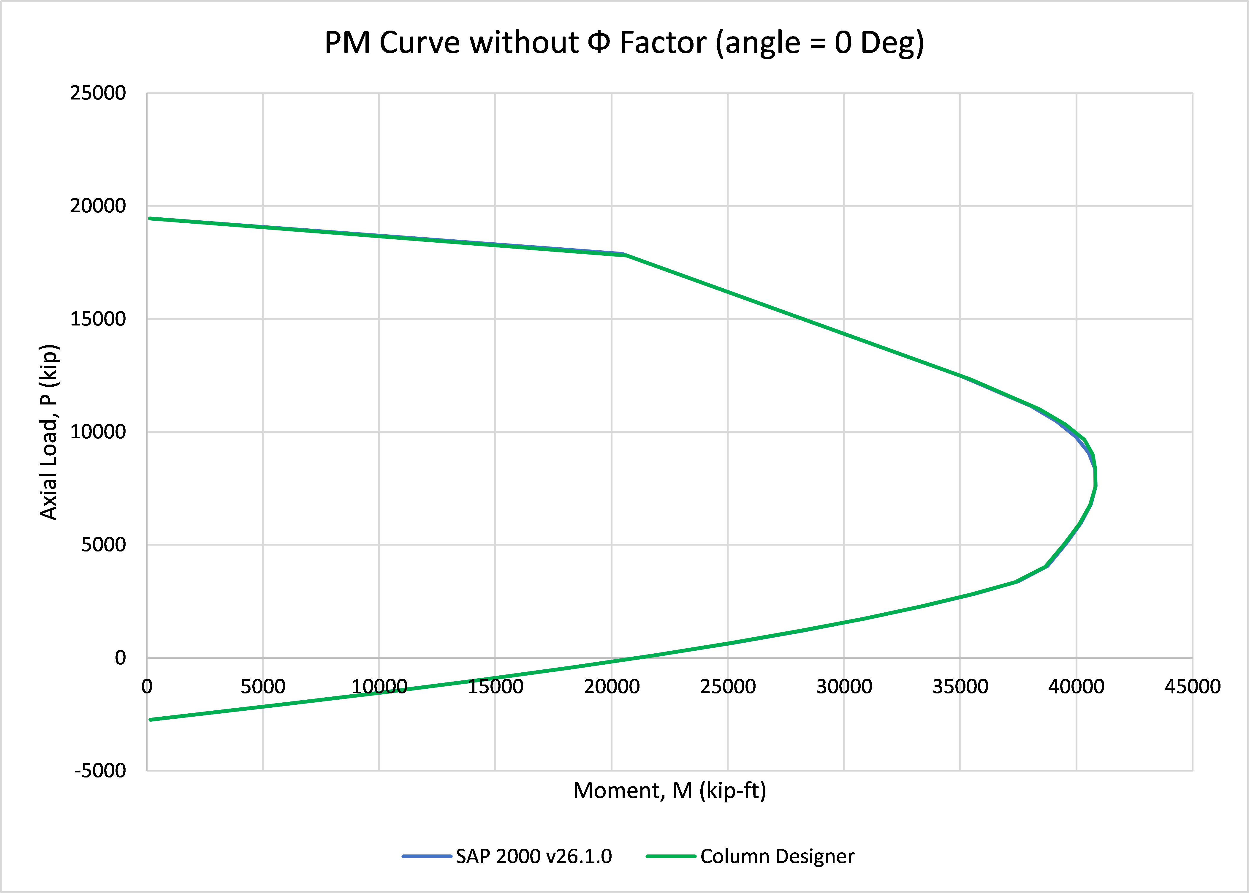
P-M INTERACTION COMPARISON WITH Ф FACTOR
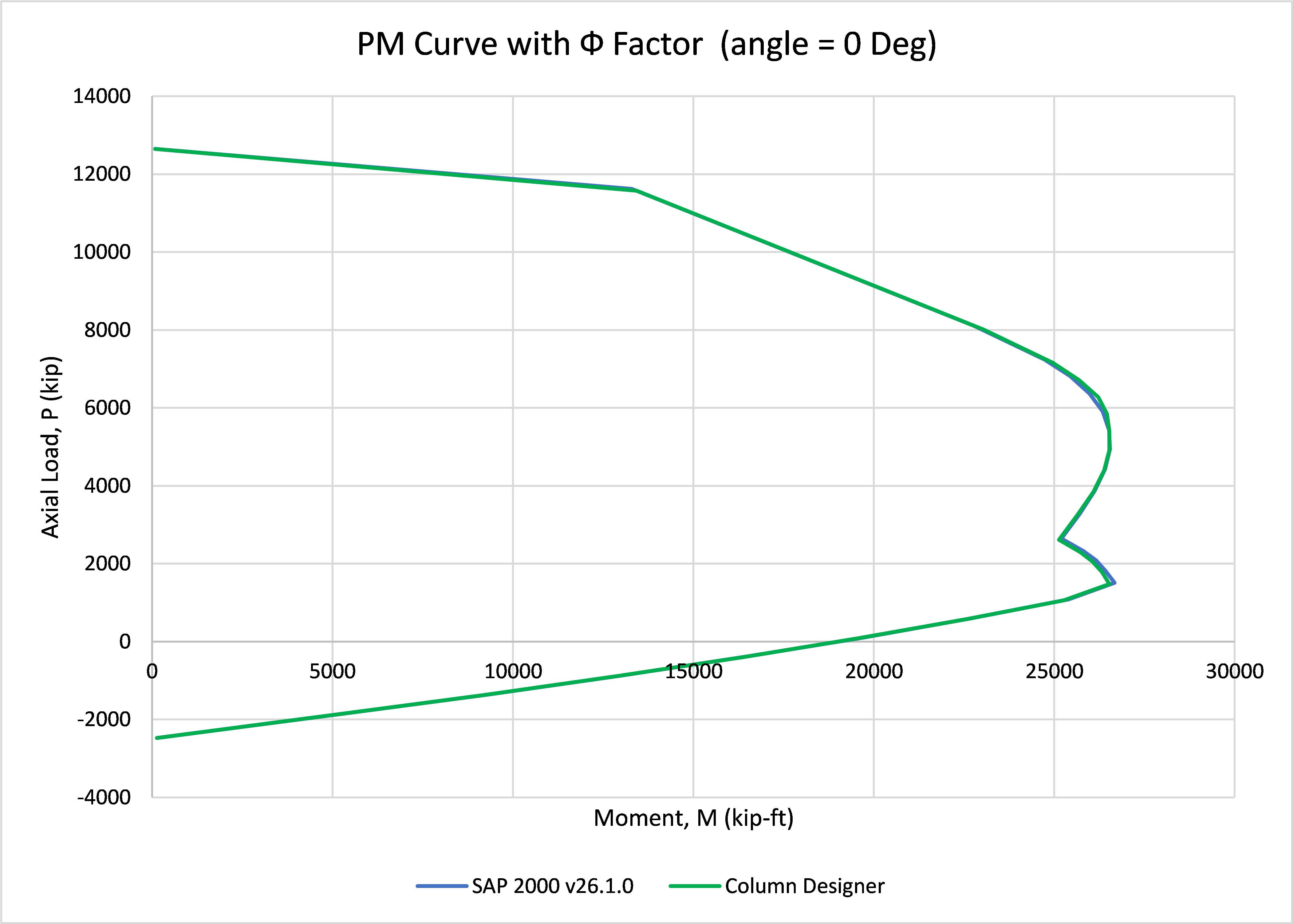
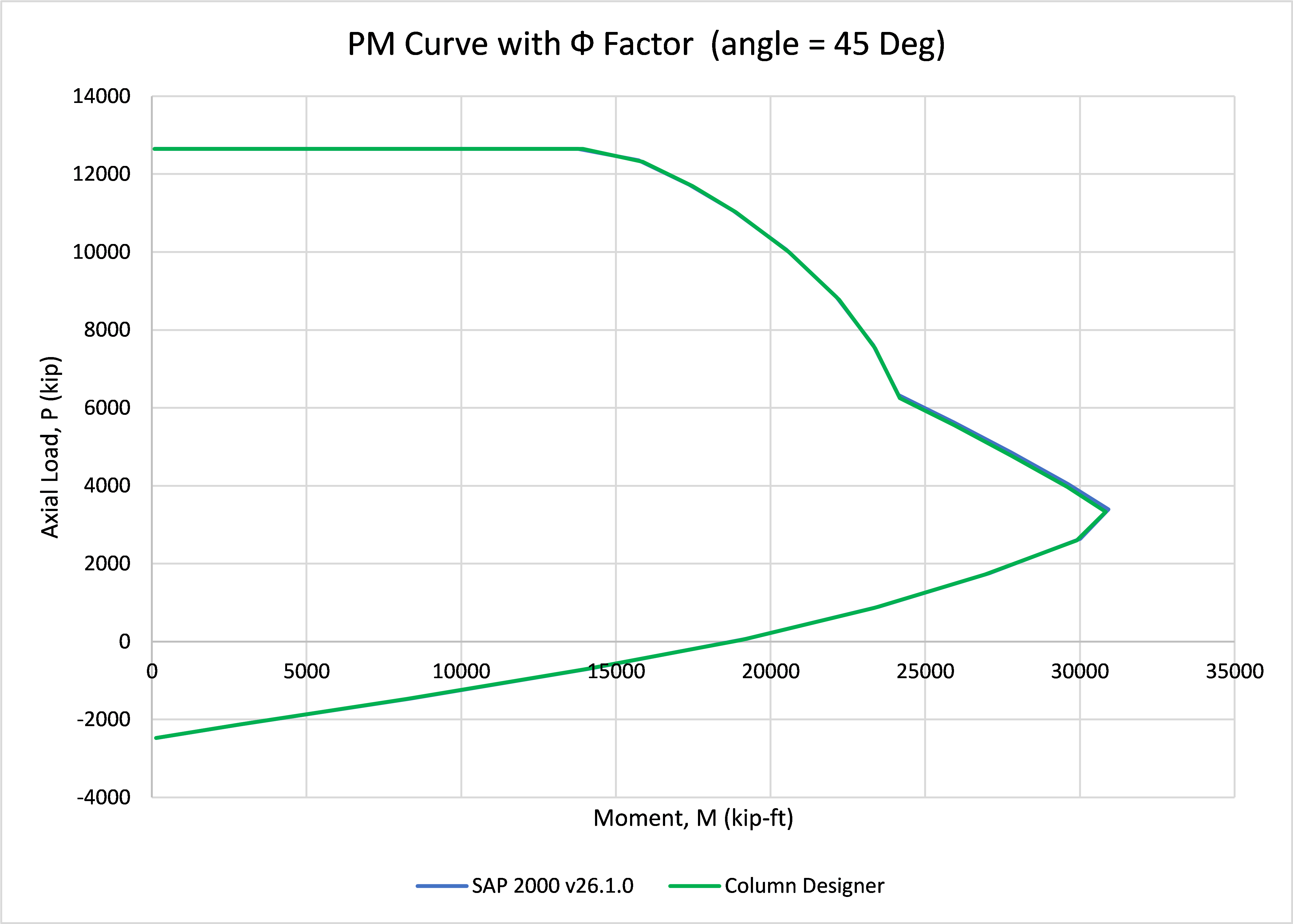
P-M INTERACTION COMPARISON WITH Ф FACTOR
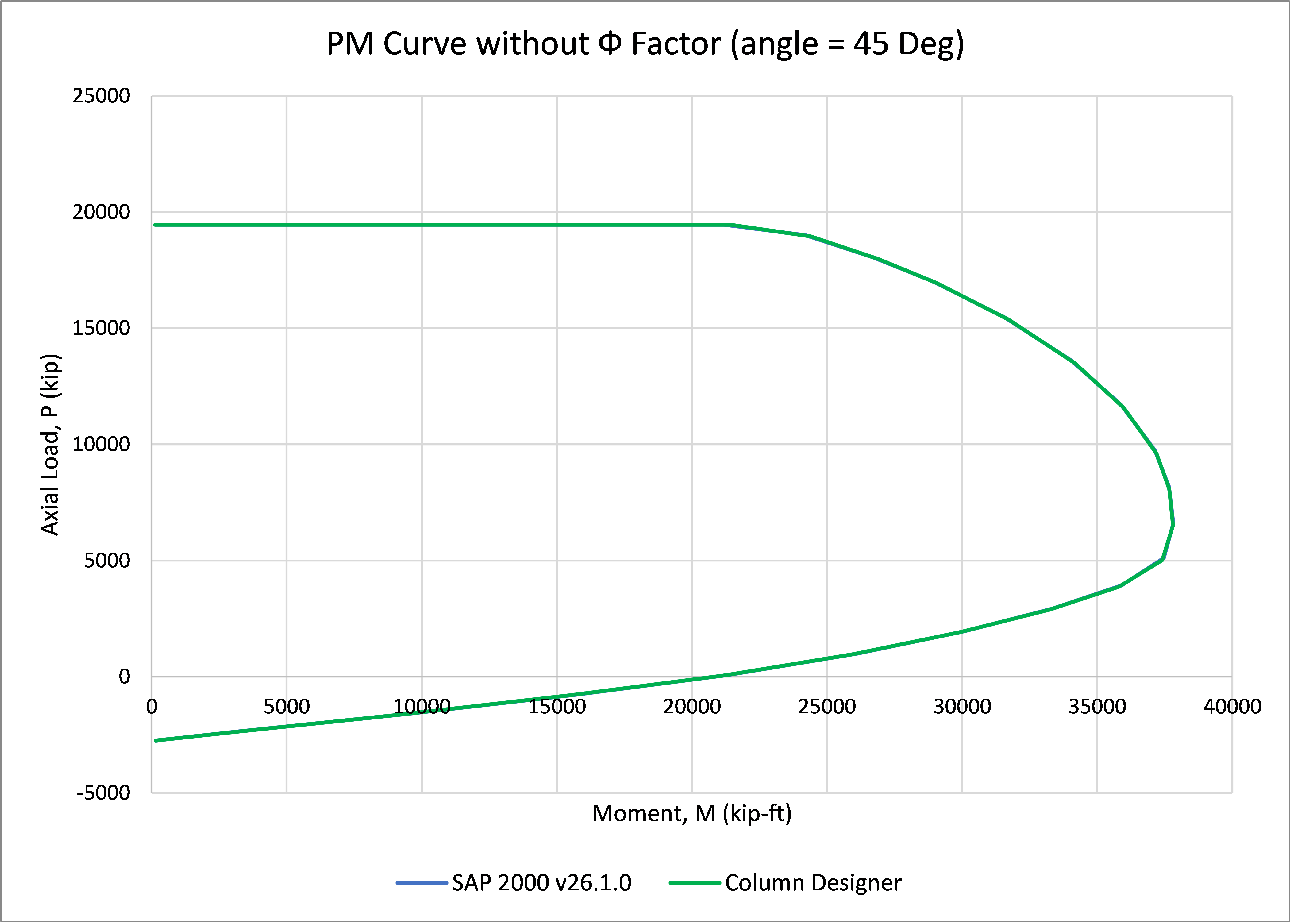
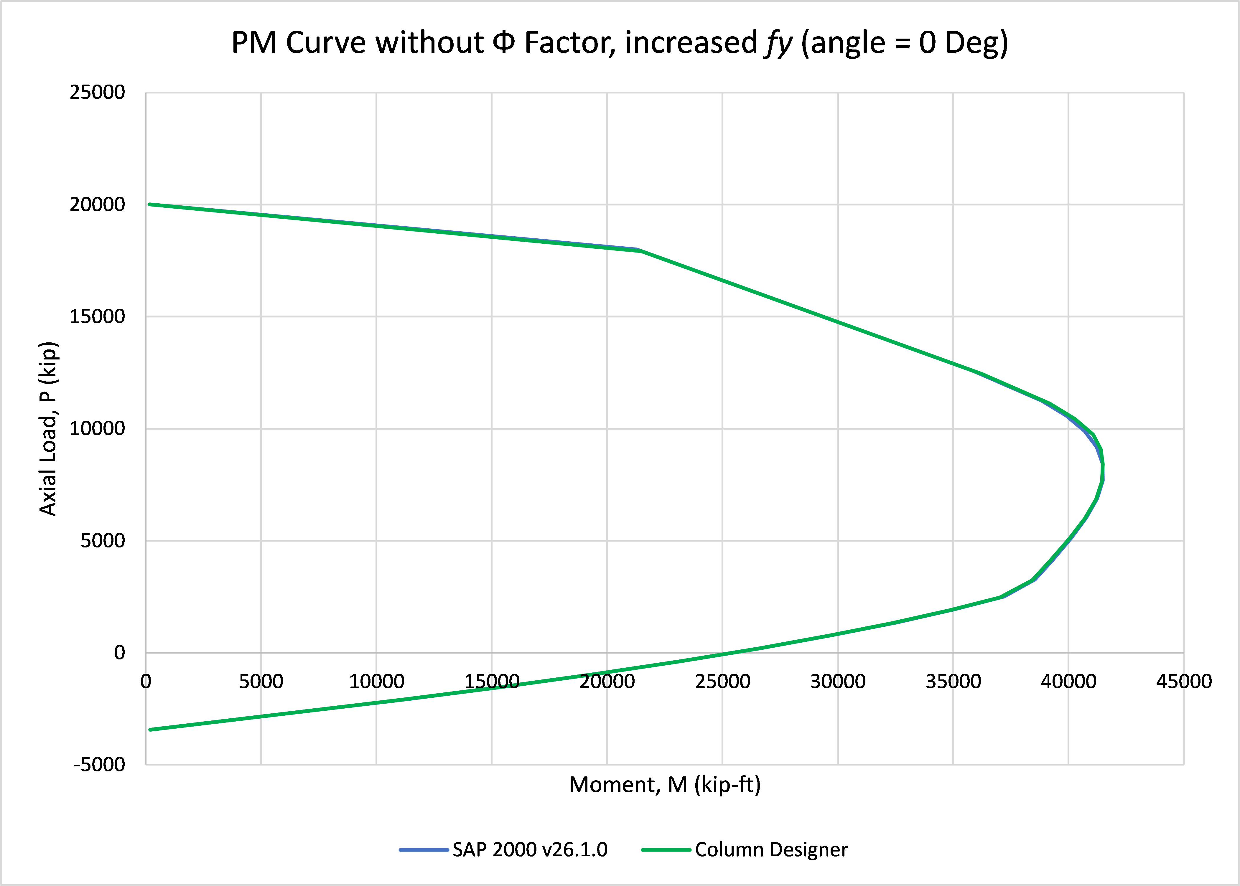
P-M INTERACTION COMPARISON WITHOUT Ф FACTOR AND INCREASED FY
Moment Magnification – Non-Sway
ACI 318-19 Moment Magnification Non-Sway- Example 001
Moment Magnification Calculation for Slender Column (Non-Sway)
GEOMETRY, PROPERTIES AND LOADING
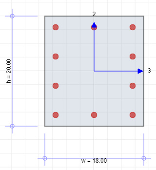
The moment magnification calculation for a given rectangular section using ACI 318-19 is tested in this example by comparing the results with manual calculation.
The column section details are as tabulated below.
Note: Refer ACI 318-19 Moment Magnification NS Ex001.cdbx
|
Parameters | Value |
|---|---|---|
| Width (in) | 18 | |
| Height (in) | 20 | |
| Compressive Strength, fc’ (psi) | 4,000 | |
| Modulus of Elasticity of Concrete, Ec (ksi) | 3,600 | |
| Minimum Yield Stress, fy (psi) | 40,000 | |
| Modulus of Elasticity of Steel, Es (ksi) | 29,000 | |
| Rebar Layout | 10-#8 | |
| Rebar Area (in2) | 7.85 | |
| Rebar Ratio | 2.18% | |
| Clear Cover (in) | 1.5 | |
| Unsupported Length, lu (ft) | 16 | |
| k-factor, braced (XZ Plane) | 0.77 | |
| k-factor, braced (YZ Plane) | 0.83 |
| Name | Axial Load, Pu (kip) | Moment Top, Mux (kip-ft) | Moment Top, Muy (kip-ft) | Moment Bottom, Mux (kip-ft) | Moment Bottom, Muy (kip-ft) | Sustained Load |
|---|---|---|---|---|---|---|
| Combination 1 | 200 | 82 | 185 | 86 | 157 | 100 |
MOMENT MAGNIFICATION COMPARISON
Column Designer reports both the top and bottom magnified moments in X and Y direction. The higher of the top and bottom magnified moments is reported as M2 while the lower magnified moment is reported as M1.
| Magnified Moments (kip-ft) | Column Designer | By hand | % Difference |
|---|---|---|---|
| M1x | 85.35 | 85.34 | 0.01% |
| M2x | 89.51 | 89.50 | 0.01% |
| M1y | 157.00 | 157.00 | 0.00% |
| M2y | 185.00 | 185.00 | 0.00% |
MANUAL CALCULATION
| Calculation of Magnified Moment about X-axis | ||||
|---|---|---|---|---|
| Loading Data | ||||
| M1 (Lower Moment) | = | 984 | kip-in | |
| M2 (Higher Moment) | = | 1,032 | kip-in | |
| Axial Load, Pu | = | 200 | kip | |
| Calculation of Critical Buckling Load | ||||
| k-factor | = | 0.83 | ||
| Unsupported Length, lu | = | 192 | in | |
| Ec | = | 3,600 | ksi | |
| (Ig)column | = | \[\frac{18*20^{3}}{12}\] | in4 | |
| = | 12,000 | in4 | ||
| 0.2EcIg | = | 8,640,000 | kip-in2 | |
| Es | = | 29,000 | ksi | |
| Ise | = | 324.42 | in4 | |
| βdns | = | 0.5 | ||
| (EI)eff | = | \[\frac{0.2E_{c}I_{g} + E_{s}I_{se}}{1 + \beta_{dns}}\] | kip-in2 | [ACI 318-19 6.6.4.4.4] |
| = | 12,032,197.01 | kip-in2 | ||
| Critical Buckling Load, Pc | = | \[\frac{\pi^{2}{(EI)}_{eff}}{{(kl_{u})}^{2}}\] | kip | [ACI 318-19 6.6.4.4.2] |
| = | 4,676.12 | kip | ||
| Calculation of Cm | ||||
| Cm | = | \[0.6 - 0.4\frac{M_{1}}{M_{2}}\] | ≥0.4 |
\[\lbrack\frac{M_{1}}{M_{2}} = - ve\ for\ single\ curvature\rbrack\] [ACI 318-19 6.6.4.5.3] |
| = | 0.98 | |||
| Calculation of Magnification Factor | ||||
| δ | = | \[\frac{C_{m}}{1 - \frac{P_{u}}{0.75P_{c}}}\] | [ACI 318-19 6.6.4.5.2] | |
| = | 1.04 | |||
| Calculation of Magnified Moment | ||||
| M1x | = | 1,024.09 | kip-in | |
| = | 85.34 | kip-ft | ||
| M2x | = | 1,074.05 | kip-in | |
| = | 89.50 | kip-ft | ||
| Calculation of Magnified Moment about Y-axis | ||||
| Loading Data | ||||
| M1 (Lower Moment) | = | 1,884 | kip-in | |
| M2 (Higher Moment) | = | 2,220 | kip-in | |
| Axial Load, Pu | = | 200 | kip | |
| Calculation of Critical Buckling Load | ||||
| k-factor | = | 0.77 | ||
| Unsupported Length, lu | = | 192 | in | |
| Ec | = | 3,600 | ksi | |
| (Ig)column | = | \[\frac{20*18^{3}}{12}\] | in4 | |
| = | 9,720 | in4 | ||
| 0.2EcIg | = | 6,998,400 | kip-in2 | |
| Es | = | 29,000 | ksi | |
| Ise | = | 308.37 | in4 | |
| βdns | = | 0.5 | ||
| (EI)eff | = | \[\frac{0.2E_{c}I_{g} + E_{s}I_{se}}{1 + \beta_{dns}}\] | kip-in2 | [ACI 318-19 6.6.4.4.4] |
| = | 10,627,361.11 | kip-in2 | ||
| Critical Buckling Load, Pc | = | \[\frac{\pi^{2}{(EI)}_{eff}}{{(kl_{u})}^{2}}\] | kip | [ACI 318-19 6.6.4.4.2] |
| = | 4,798.90 | kip | ||
| Calculation of Cm | ||||
| Cm | = | \[0.6 - 0.4\frac{M_{1}}{M_{2}}\] | ≥0.4 |
\[\lbrack\frac{M_{1}}{M_{2}} = - ve\ for\ single\ curvature\rbrack\] [ACI 318-19 6.6.4.5.3] |
| = | 0.94 | |||
| Calculation of Magnification Factor | ||||
| δ | = | \[\frac{C_{m}}{1 - \frac{P_{u}}{0.75P_{c}}}\] | [ACI 318-19 6.6.4.5.2] | |
| = | 1 | |||
| Calculation of Magnified Moment | ||||
| M1y | = | 1,884.00 | kip-in | |
| = | 157.00 | kip-ft | ||
| M2y | = | 2,220.00 | kip-in | |
| = | 185.00 | kip-ft | ||
ACI 318-19 Moment Magnification Non-Sway- Example 002
Moment Magnification Calculation for Slender Column (Non-Sway)
GEOMETRY, PROPERTIES AND LOADING
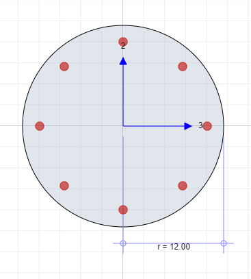
The moment magnification calculation for a given circular section using ACI 318-19 is tested in this example by comparing the results with manual calculation.
The column section details are as tabulated below.
Note: Refer ACI 318-19 Moment Magnification NS Ex002.cdbx
|
Parameters | Value |
|---|---|---|
| Diameter (in) | 24 | |
| Compressive Strength, fc’ (psi) | 4,000 | |
| Modulus of Elasticity of Concrete, Ec (ksi) | 3,600 | |
| Minimum Yield Stress, fy (psi) | 40,000 | |
| Modulus of Elasticity of Steel, Es (ksi) | 29,000 | |
| Rebar Layout | 8-#9 | |
| Rebar Area (in2) | 7.99 | |
| Rebar Ratio | 1.77% | |
| Clear Cover (in) | 1.5 | |
| Unsupported Length, lu (ft) | 18 | |
| k-factor, braced (XZ Plane) | 0.71 | |
| k-factor, braced (YZ Plane) | 0.84 |
| Name | Axial Load, Pu (kip) | Moment Top, Mux (kip-ft) | Moment Top, Muy (kip-ft) | Moment Bottom, Mux (kip-ft) | Moment Bottom, Muy (kip-ft) | Sustained Load |
|---|---|---|---|---|---|---|
| Combination 1 | 600 | 210 | 95 | 85 | 70 | 400 |
MOMENT MAGNIFICATION COMPARISON
Column Designer reports both the top and bottom magnified moments in X and Y direction. The higher of the top and bottom magnified moments is reported as M2 while the lower magnified moment is reported as M1.
| Magnified Moments (kip-ft) | Column Designer | By hand | % Difference |
|---|---|---|---|
| M1x | 85.00 | 85.00 | 0.00% |
| M2x | 210.00 | 210.00 | 0.00% |
| M1y | 72.59 | 72.58 | 0.01% |
| M2y | 98.51 | 98.50 | 0.01% |
MANUAL CALCULATION
|
Calculation of Magnified Moment about X-axis
|
||||
|---|---|---|---|---|
| Loading Data | ||||
| M1 (Lower Moment) | = | 1020 | kip-in | |
| M2 (Higher Moment) | = | 2520 | kip-in | |
| Axial Load, Pu | = | 600 | kip | |
| Calculation of Critical Buckling Load | ||||
| k-factor | = | 0.84 | ||
| Unsupported Length, lu | = | 216 | in | |
| Ec | = | 3600 | ksi | |
| (Ig)column | = | \[\frac{\pi*12^{4}}{4}\] | in4 | |
| = | 16,286.02 | in4 | ||
| 0.2EcIg | = | 11,725,931.75 | kip-in2 | |
| Es | = | 29,000 | ksi | |
| Ise | = | 395.27 | in4 | |
| βdns | = | 0.67 | ||
| (EI)eff | = | \[\frac{0.2E_{c}I_{g} + E_{s}I_{se}}{1 + \beta_{dns}}\] | kip-in2 | [ACI 318-19 6.6.4.4.4] |
| = | 13,913,201.38 | kip-in2 | ||
| Critical Buckling Load, Pc | = | \[\frac{\pi^{2}{(EI)}_{eff}}{{(kl_{u})}^{2}}\] | kip | [ACI 318-19 6.6.4.4.2] |
| = | 4,171.20 | kip | ||
| Calculation of Cm | ||||
| Cm | = | \[0.6 - 0.4\frac{M_{1}}{M_{2}}\] | ≥0.4 |
\[\lbrack\frac{M_{1}}{M_{2}} = - ve\ for\ single\ curvature\rbrack\] [ACI 318-19 6.6.4.5.3] |
| = | 0.76 | |||
| Calculation of Magnification Factor | ||||
| δ | = | \[\frac{C_{m}}{1 - \frac{P_{u}}{0.75P_{c}}}\] | [ACI 318-19 6.6.4.5.2] | |
| = | 1 | |||
| Calculation of Magnified Moment | ||||
| M1x | = | 1,020.00 | kip-in | |
| = | 85.00 | kip-ft | ||
| M2x | = | 2,520.00 | kip-in | |
| = | 210.00 | kip-ft | ||
| Calculation of Magnified Moment about Y-axis | ||||
|---|---|---|---|---|
| Loading Data | ||||
| M1 (Lower Moment) | = | 840 | kip-in | |
| M2 (Higher Moment) | = | 1,140 | kip-in | |
| Axial Load, Pu | = | 600 | kip | |
| Calculation of Critical Buckling Load | ||||
| k-factor | = | 0.71 | ||
| Unsupported Length, lu | = | 216 | in | |
| Ec | = | 3,600 | ksi | |
| (Ig)column | = | \[\frac{\pi*12^{4}}{4}\] | in4 | |
| = | 16,286.02 | in4 | ||
| 0.2EcIg | = | 11,725,931.75 | kip-in2 | |
| Es | = | 29,000 | ksi | |
| Ise | = | 395.27 | in4 | |
| βdns | = | 0.67 | ||
| (EI)eff | = | \[\frac{0.2E_{c}I_{g} + E_{s}I_{se}}{1 + \beta_{dns}}\] | kip-in2 | [ACI 318-19 6.6.4.4.4] |
| = | 13,913,201.38 | kip-in2 | ||
| Critical Buckling Load, Pc | = | \[\frac{\pi^{2}{(EI)}_{eff}}{{(kl_{u})}^{2}}\] | kip | [ACI 318-19 6.6.4.4.2] |
| = | 5,838.52 | kip | ||
| Calculation of Cm | ||||
| Cm | = | \[0.6 - 0.4\frac{M_{1}}{M_{2}}\] | ≥0.4 |
\[\lbrack\frac{M_{1}}{M_{2}} = - ve\ for\ single\ curvature\rbrack\] [ACI 318-19 6.6.4.5.3] |
| = | 0.89 | |||
| Calculation of Magnification Factor | ||||
| δ | = | \[\frac{C_{m}}{1 - \frac{P_{u}}{0.75P_{c}}}\] | [ACI 318-19 6.6.4.5.2] | |
| = | 1.04 | |||
| Calculation of Magnified Moment | ||||
| M1y | = | 870.91 | kip-in | |
| = | 72.58 | kip-ft | ||
| M2y | = | 1,181.95 | kip-in | |
| = | 98.50 | kip-ft | ||
Eurocode 2-2004 Moment Magnification Non-Sway- Example 001
Moment Magnification Calculation for Slender Column (Non-Sway)
GEOMETRY, PROPERTIES AND LOADING
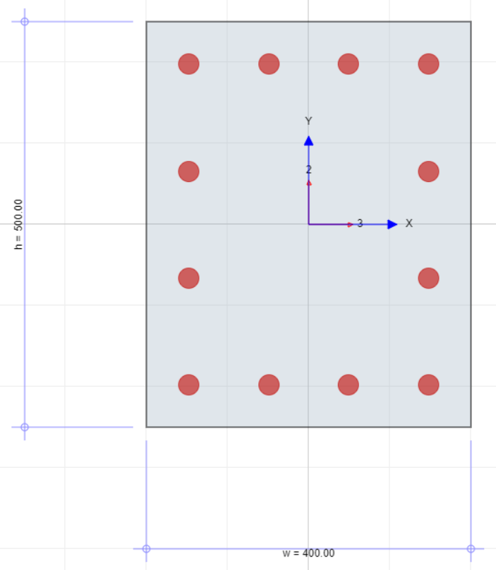
The moment magnification calculation for a given rectangular section using Eurocode 2:2004 is tested in this example by comparing the results with manual calculation.
The column section details are as tabulated below.
Note: Refer Eurocode 2-2004 Moment Magnification NS Ex001.cdbx
|
Parameters | Value |
|---|---|---|
| Width, w (mm) | 400 | |
| Height, h (mm) | 500 | |
| Rebar Layout | 12-d25 | |
| Clear Cover, cc (mm) | 40 | |
| Compressive Strength, fck (MPa) | 40 | |
| Minimum Yield Stress, fyk (MPa) | 500 | |
| Modulus of Elasticity of Concrete, Ec (MPa) | 35,000 | |
| Modulus of Elasticity of Steel, Es (MPa) | 200,000 | |
| Concrete Area, Ac (mm2) | 200,000 | |
| Rebar Area, As (mm2) | 5,890.49 | |
| Concrete Inertia, Ig, 22 (mm4) | 2.667x10⁹ | |
| Concrete Inertia, Ig, 33 (mm4) | 4.167x10⁹ | |
| Rebar Inertia, Is, 22 (mm4) | 9.018 x10⁷ | |
| Rebar Inertia, Is, 33 (mm4) | 1.617x10⁸ | |
| Perimeter, u (mm) | 1,800 | |
| Relative Humidity, RH (%) | 50 | |
| Ratio SLS to ULS moments, rm | 0.8 | |
| Age of concrete at loading, t0 (days) | 28 | |
| Concrete partial safety factor, γc | 1.5 | |
| Reinforcing partial safety factor, γs | 1.15 | |
| Long term compressive strength factor, αcc | 1 | |
| Unsupported Length, lu (m) | 3 | |
| Effective Length Factor (Braced), kXZ | 0.89 | |
| Effective Length Factor (Braced), kYZ | 0.94 | |
| Biaxial Loading | Yes |
| Name | Axial Load, NEd (kN) |
Moment Top, Mx,top (kN-m) |
Moment Top, My,top (kN-m) |
Moment Bottom, Mx,bot (kN-m) |
Moment Bottom, My,bot (kN-m) |
|---|---|---|---|---|---|
| Combination 1 | 1000 | 110 | 250 | 120 | 210 |
MOMENT MAGNIFICATION COMPARISON
Column Designer reports both the design moments in X and Y direction. The design moments are reported as the top moments for capacity calculations, while the bottom moments remain unchanged.
| Design Moments (kN-m) | Column Designer | By hand | % Difference |
|---|---|---|---|
| \(M_{Ed,x}\) | 150.98 | 150.97 | 0.01% |
| \(M_{Ed,y}\) | 270.86 | 270.87 | 0.01% |
| \(M_{c}\) | 371.03 | 371.03 | 0.00% |
MANUAL CALCULATION
| Calculation of Design Moment about X-axis | ||||
|---|---|---|---|---|
| Loading Data | ||||
| Moment Top, Mx, top | = | 110,000,000 | N-mm | |
| Moment Bottom, Mx, bot | = | 120,000,000 | N-mm | |
| Axial Load, NEd | = | 1,000,000 | N | |
| Calculation of Additional Parameters | ||||
| Effective Length, l0 | = | kYZ × lu | [EC2 5.8.3.2 (3)] | |
| = | 0.94×3,000 | |||
| = | 2820 | mm | ||
| Design Compressive Strength, fcd | = | \[\alpha_{cc} \times \frac{f_{ck}}{\gamma_{c}}\] | [EC2 3.1.6 (1)] | |
| = | 1×40⁄1.5 | |||
| = | 26.67 | MPa | ||
| Mean Value Cylinder Compressive Strength, fcm | = | fck + 8 | [EC2 Table 3.1] | |
| = | 40+8 | |||
| = | 48 | MPa | ||
| Design Yield Strength, fyd | = | \[\frac{f_{yk}}{\gamma_{s}}\] | [EC2 3.2.7 (2)] | |
| = | 500⁄1.15 | |||
| = | 434.78 | MPa | ||
| Design Strain, εyd | = | \[\frac{f_{yd}}{E_{s}}\] | [EC2 5.8.8.3 (1)] | |
| = | 434.78⁄200000 | |||
| = | 0.002174 | mm/mm | ||
| Curvature Distribution Factor, c | = | 10 | [EC2 5.8.8.2 (4)] | |
| Radius of Gyration of Concrete Section, rc | = | \[\sqrt{\frac{I_{g,33}}{A_{c}}}\] | ||
| = | \[\sqrt{\frac{4.167 \times 10^{9}}{200,000}}\] | |||
| = | 144.34 | mm | ||
| Radius of Gyration of Rebar, rs | = | \[\sqrt{\frac{I_{s,33}}{A_{s}}}\] | ||
| = | \[\sqrt{\frac{1.617 \times 10^{8}}{5,890.49}}\] | |||
| = | 165.68 | mm | ||
| Effective Depth, d | = | \[\frac{h}{2} + r_{s}\] | [EC2 5.8.8.3 (2)] | |
| = | 500⁄2+165.68 | |||
| = | 415.68 | mm | ||
| Determine First Order End Moments | ||||
| Determine M01 and M02 to satisfy |M02| ≥ |M01| | [EC2 5.8.8.2 (2)] | |||
|
NOTE:
|
[IStructE Manual EC2 5.5.4.2] | |||
| Lower End Moment, M01 | = | min {Mx, top, Mx, bot} | ||
| = | 110,000,000 | N-mm | ||
| Higher End Moment, M02 | = | max {Mx, top, Mx, bot} | ||
| = | 120,000,000 | N-mm | ||
| Calculate Curvature | ||||
| Mechanical Reinforcement Ratio, ω | = | \[\frac{A_{s} \times f_{yd}}{A_{c} \times f_{cd}}\\] | [EC2 5.8.8.3 (3)] | |
| = | (5,890.49×434.78)/(200,000×26.67) | |||
| = | 0.4801 | |||
| Relative Ultimate Axial Load, nu | = | 1+ω | [EC2 5.8.8.3 (3)] | |
| = | 1+0.4801 | |||
| = | 1.4801 | |||
| Relative Axial Force, n | = | \[\frac{N_{Ed}}{\left( A_{c} \times f_{cd} \right)}\] | [EC2 5.8.8.3 (3)] | |
| = | 1,000,000⁄((200,000×26.67)) | |||
| = | 0.1875 | |||
| Relative Balanced Load, nbal | = | 0.4 | [EC2 5.8.8.3 (3)] | |
| Axial Load Correction Factor, Kr | = | \[\frac{nu - n}{nu - n_{bal}} \leq 1\] | [EC2 5.8.8.3 (3)] | |
| = | \[\frac{1.4801 - 0.4}{1.4801 - 0.1875} \leq 1\] | |||
| = | 1 | |||
| Member Notional Size, h0 | = | \[\frac{2 \times A_{c}}{u}\] | [EC2 Annex B.1 (1) Eqn(B.6)] | |
| = | (2×200,000)/1800 | |||
| = | 222.22 | mm | ||
| Influence of Concrete Strength Coefficient, α1 | = | \[\left( \frac{35}{f_{cm}} \right)^{0.7}\] | [EC2 Annex B.1 (1) Eqn(B.8c)] | |
| = | (35⁄48)0.7 | |||
| = | 0.8016 | |||
| Influence of Concrete Strength Coefficient, α2 | = | \[\left( \frac{35}{f_{cm}} \right)^{0.2}\] | [EC2 Annex B.1 (1) Eqn(B.8c)] | |
| = | (35⁄48)0.2 | |||
| = | 0.9388 | |||
| Factor for Effect of Relative Humidity on Notional Creep Coefficient, φRH | [EC2 Annex B.1 (1) Eqn(B.3)] | |||
|
NOTE:
|
||||
| φRH | = | \[\left\lbrack 1 + \left( \frac{1 - \frac{RH}{100}}{0.1 \times \sqrt[3]{h_{0}}} \times \alpha_{1} \right) \right\rbrack \times \alpha_{2}\] | ||
| = | \[\left\lbrack 1 + \left( \frac{1 - \frac{50}{100}}{0.1 \times \sqrt[3]{222.22}} \times 0.8016 \right) \right\rbrack \times 0.9388\] | |||
| = | 1.56 | |||
| Factor for Effect of Concrete Strength on Notional Creep Coefficient, β(fcm) | = | \[\frac{16.8}{\sqrt{f_{cm}}}\] | [EC2 Annex B.1 (1) Eqn(B.4)] | |
| = | \[\frac{16.8}{\sqrt{48}}\] | |||
| = | 2.425 | |||
| Factor for Effect of Concrete Age on Notional Creep Coefficient, β(t0) | = | 1/ (0.1+t00.2) | [EC2 Annex B.1 (1) Eqn(B.5)] | |
| = | 1/ (0.1+280.2) | |||
| = | 0.4884 | |||
| Notional Creep Coefficient, φ0 | = | φRH × β(fcm) × β(t0) | [EC2 Annex B.1 (1) Eqn(B.2)] | |
| = | 1.56×2.425×0.4884 | |||
| = | 1.848 | |||
| Effective Creep Ratio, φef | = | φ0 × rm | [EC2 5.8.4 (2)] | |
| = | 1.848×0.8 | |||
| = | 1.4784 | |||
| Slenderness Ratio, λ | = | \[\frac{l_{0}}{r}_{c}\] | [EC2 5.8.3.2 (1)] | |
| = | 2820⁄144.34 | |||
| = | 19.54 | |||
| Factor, β | = | \[0.35 + \frac{f_{ck}}{200} - \frac{\lambda}{150}\] | [EC2 5.8.8.3 (4)] | |
| = | 0.35+40⁄200-19.54⁄150 | |||
| = | 0.4197 | |||
| Creep Factor, Kφ | = | 1 + β × φef ≥ 1 | [EC2 5.8.8.3 (4)] | |
| = | 1 + 0.4197 × 1.4784 ≥ 1 | |||
| = | 1.6205 | |||
| Curvature, \(\frac{1}{r}\) | = | \[K_{r} \times K_{\varphi} \times \frac{\varepsilon_{yd}}{0.45d}\] | [EC2 5.8.8.3 (1)] | |
| = | 1×1.6205×0.002174/0.45(415.68) | |||
| = | 0.00001883 | 1/mm | ||
| Calculate Moment due to Geometric Imperfections | ||||
| Eccentricity due to Geometric Imperfections, ei | = | \[\max\left\{ \frac{l_{0}}{400},\frac{h}{30},20 \right\}\] | [EC2 5.2 (7)a] | |
| = | \[\max\left\{ \frac{2820}{400},\frac{500}{30},20 \right\}\] | [EC2 6.1 (4)] | ||
| = | 20 | mm | ||
| Geometric Imperfections Moment, Mi | = | NEd × ei | [EC2 5.2 (7) Fig 5.1a] | |
| = | 1,000,000×20 | |||
| = | 20,000,000 | N-mm | ||
| Calculate First Order Moment | ||||
| First Order Moment, M0e | = | 0.6M02 + 0.4M01 ≥ 0.4M02 | [EC2 5.8.8.2 (2)] | |
| = | 0.6 × 120, 000, 000 + 0.4 × 110000, 000 ≥ 0.4 × 120000000 | |||
| = | 116,000,000 | N-mm | ||
| Included Effect of Imperfections, M0Ed | = | M0e+Mi | [EC2 5.8.8.2 (1)] | |
| = | 116,000,000+20,000,000 | |||
| = | 136000000 | N-mm | ||
| Calculate Nominal Second Order Moment | ||||
| Deflection, e2 | = | \[\left( \frac{1}{r} \right) \times {l_{0}}^{2}/c\] | [EC2 5.8.8.2 (3)] | |
| = | 0.00001883×28202/10 | |||
| = | 14.974 | mm | ||
| Nominal Second Order Moment, M2 | = | NEd × e2 | [EC2 5.8.8.2 (3)] | |
| = | 1,000,000×14.974 | |||
| = | 14,974,000 | N-mm | ||
| Calculate Design Moment | ||||
| The design moment is the maximum of: | ||||
|
= | 120 | kN-m | [EC2 5.8.8.2 (1)] |
|
= | 136+14.974 | [Concise EC2 5.6.2.2] | |
| = | 150.97 | kN-m | ||
|
= | 110+0.5×14.974 | ||
| = | 117.487 | kN-m | ||
|
= | 1,000×max(400/30,2) | ||
| = | 20 | kN-m | ||
| Design Moment, MEd, x | = | \[\max\left\{ M_{02},M_{0Ed} + M_{2},M_{01} + 0.5M_{2},N_{Ed} \times \max\left( \frac{b}{30},20 \right) \right\}\] | ||
| = | 150.97 | kN-m | ||
| Calculation of Design Moment about Y-axis | ||||
| Loading Data | ||||
| Moment Top, My, top | = | 250,000,000 | N-mm | |
| Moment Bottom, My, bot | = | 210,000,000 | N-mm | |
| Axial Load, NEd | = | 1,000,000 | N | |
| Calculation of Additional Parameters | ||||
| Effective Length, l0 | = | kXZ × lu | [EC2 5.8.3.2 (3)] | |
| = | 0.89×3,000 | |||
| = | 2670 | mm | ||
| Design Compressive Strength, fcd | = | \[\alpha_{cc} \times \frac{f_{ck}}{\gamma_{c}}\] | [EC2 3.1.6 (1)] | |
| = | 1×40/1.5 | |||
| = | 26.67 | MPa | ||
| Mean Value Cylinder Compressive Strength, fcm | = | fck+8 | [EC2 Table 3.1] | |
| = | 40+8 | |||
| = | 48 | MPa | ||
| Design Yield Strength, fyd | = | \[\frac{f_{yk}}{\gamma_{s}}\] | [EC2 3.2.7 (2)] | |
| = | 500/1.15 | |||
| = | 434.78 | MPa | ||
| Design Strain, εyd | = | \[\frac{f_{yd}}{E_{s}}\] | [EC2 5.8.8.3 (1)] | |
| = | 434.78/200,000 | |||
| = | 0.002174 | mm/mm | ||
| Curvature Distribution Factor, c | = | 10 | [EC2 5.8.8.2 (4)] | |
| Radius of Gyration of Concrete Section, rc | = | \[\sqrt{\frac{I_{g,33}}{A_{c}}}\] | ||
| = | \[\sqrt{\frac{2.667 \times 10^{9}}{200,000}}\] | |||
| = | 115.48 | mm | ||
| Radius of Gyration of Rebar, rs | = | \[\sqrt{\frac{I_{s,33}}{A_{s}}}\] | ||
| = | \[\sqrt{\frac{9.018 \times 10^{7}}{5,890.49}}\] | |||
| = | 123.73 | mm | ||
| Effective Depth, d | = | w/2+rs | [EC2 5.8.8.3 (2)] | |
| = | 400/2+123.73 | |||
| = | 323.73 | mm | ||
| Determine First Order End Moments | ||||
| Determine M01 and M02 to satisfy |M02| ≥ |M01| | [EC2 5.8.8.2 (2)] | |||
|
NOTE:
|
[IStructE Manual EC2 5.5.4.2] | |||
| Lower End Moment, M01 | = | min {My, top, My, bot} | ||
| = | 210,000,000 | N-mm | ||
| Higher End Moment, M02 | = | max {My, top, My, bot} | ||
| = | 250,000,000 | N-mm | ||
| Calculate Curvature | ||||
| Mechanical Reinforcement Ratio, ω | = | \[\frac{A_{s} \times f_{yd}}{A_{c} \times f_{cd}}\\] | [EC2 5.8.8.3 (3)] | |
| = | (5,890.49×434.78)/(200,000×26.67) | |||
| = | 0.4801 | |||
| Relative Ultimate Axial Load, nu | = | 1+ω | [EC2 5.8.8.3 (3)] | |
| = | 1+0.4801 | |||
| = | 1.4801 | |||
| Relative Axial Force, n | = | \[\frac{N_{Ed}}{\left( A_{c} \times f_{cd} \right)}\] | [EC2 5.8.8.3 (3)] | |
| = | 1,000,000/(200,000×26.67) | |||
| = | 0.1875 | |||
| Relative Balanced Load, nbal | = | 0.4 | [EC2 5.8.8.3 (3)] | |
| Axial Load Correction Factor, Kr | = | \[\frac{nu - n}{nu - n_{bal}} \leq 1\] | [EC2 5.8.8.3 (3)] | |
| = | \[\frac{1.4801 - 0.4}{1.4801 - 0.1875} \leq 1\] | |||
| = | 1 | |||
| Member Notional Size, h0 | = | \[\frac{2 \times A_{c}}{u}\] | [EC2 Annex B.1 (1) Eqn(B.6)] | |
| = | (2×200,000)/1800 | |||
| = | 222.22 | mm | ||
| Influence of Concrete Strength Coefficient, α1 | = | \[\left( \frac{35}{f_{cm}} \right)^{0.7}\] | [EC2 Annex B.1 (1) Eqn(B.8c)] | |
| = | (35⁄48)0.7 | |||
| = | 0.8016 | |||
| Influence of Concrete Strength Coefficient, α2 | = | \[\left( \frac{35}{f_{cm}} \right)^{0.2}\] | [EC2 Annex B.1 (1) Eqn(B.8c)] | |
| = | (35⁄48)0.2 | |||
| = | 0.9388 | |||
| Factor for Effect of Relative Humidity on Notional Creep Coefficient, φRH | [EC2 Annex B.1 (1) Eqn(B.3)] | |||
|
NOTE:
|
||||
| φRH | = | \[\left\lbrack 1 + \left( \frac{1 - \frac{RH}{100}}{0.1 \times \sqrt[3]{h_{0}}} \times \alpha_{1} \right) \right\rbrack \times \alpha_{2}\] | ||
| = | \[\left\lbrack 1 + \left( \frac{1 - \frac{50}{100}}{0.1 \times \sqrt[3]{222.22}} \times 0.8016 \right) \right\rbrack \times 0.9388\] | |||
| = | 1.56 | |||
| Factor for Effect of Concrete Strength on Notional Creep Coefficient, β(fcm) | = | \[\frac{16.8}{\sqrt{f_{cm}}}\] | [EC2 Annex B.1 (1) Eqn(B.4)] | |
| = | \[\frac{16.8}{\sqrt{48}}\] | |||
| = | 2.425 | |||
| Factor for Effect of Concrete Age on Notional Creep Coefficient, β(t0) | = | 1/(0.1+t00.2) | [EC2 Annex B.1 (1) Eqn(B.5)] | |
| = | 1/ (0.1+280.2) | |||
| = | 0.4884 | |||
| Notional Creep Coefficient, φ0 | = | φRH × β(fcm) × β(t0) | [EC2 Annex B.1 (1) Eqn(B.2)] | |
| = | 1.56×2.425×0.4884 | |||
| = | 1.848 | |||
| Effective Creep Ratio, φef | = | φ0 × rm | [EC2 5.8.4 (2)] | |
| = | 1.848×0.8 | |||
| = | 1.4784 | |||
| Slenderness Ratio, λ | = | l0/rc | [EC2 5.8.3.2 (1)] | |
| = | 2670/115.48 | |||
| = | 23.12 | |||
| Factor, β | = | \[0.35 + \frac{f_{ck}}{200} - \frac{\lambda}{150}\] | [EC2 5.8.8.3 (4)] | |
| = | 0.35+40/200-23.12/150 | |||
| = | 0.3959 | |||
| Creep Factor, Kφ | = | 1 + β × φef ≥ 1 | [EC2 5.8.8.3 (4)] | |
| = | 1 + 0.3959 × 1.4784 ≥ 1 | |||
| = | 1.5853 | |||
| Curvature, \(\frac{1}{r}\) | = | \[K_{r} \times K_{\varphi} \times \frac{\varepsilon_{yd}}{0.45d}\] | [EC2 5.8.8.3 (1)] | |
| = | 1×1.5853×0.002174/0.45(323.73) | |||
| = | 0.00002366 | 1/mm | ||
| Calculate Moment due to Geometric Imperfections | ||||
| Eccentricity due to Geometric Imperfections, ei | = | \[\max\left\{ \frac{l_{0}}{400},\frac{w}{30},20 \right\}\] | [EC2 5.2 (7)a] | |
| = | \[\max\left\{ \frac{2670}{400},\frac{400}{30},20 \right\}\] | [EC2 6.1 (4)] | ||
| = | 20 | mm | ||
| Geometric Imperfections Moment, Mi | = | NEd × ei | [EC2 5.2 (7) Fig 5.1a] | |
| = | 1,000,000×20 | |||
| = | 20,000,000 | N-mm | ||
| Calculate First Order Moment | ||||
| First Order Moment, M0e | = | 0.6M02 + 0.4M01 ≥ 0.4M02 | [EC2 5.8.8.2 (2)] | |
| = | 0.6 × 250, 000, 000 + 0.4 × 210000000 ≥ 0.4 × 250000000 | |||
| = | 234,000,000 | N-mm | ||
| Included Effect of Imperfections, M0Ed | = | M0e + Mi | [EC2 5.8.8.2 (1)] | |
| = | 234,000,000+20,000,000 | |||
| = | 254,000,000 | N-mm | ||
| Calculate Nominal Second Order Moment | ||||
| Deflection, e2 | = | \[\left( \frac{1}{r} \right) \times {l_{0}}^{2}/c\] | [EC2 5.8.8.2 (3)] | |
| = | 0.00002366×26702/10 | |||
| = | 16.867 | mm | ||
| Nominal Second Order Moment, M2 | = | NEd × e2 | [EC2 5.8.8.2 (3)] | |
| = | 1,000,000×16.867 | |||
| = | 16,867,000 | N-mm | ||
| Calculate Design Moment | ||||
| The design moment is the maximum of: | ||||
|
= | 250 | kN-m | [EC2 5.8.8.2 (1)] |
|
= | 254+16.867 | [Concise EC2 5.6.2.2] | |
| = | 270.87 | kN-m | ||
|
= | 210+0.5×16.867 | ||
| = | 218.43 | kN-m | ||
|
= | 1,000×max (500⁄30,2) | ||
| = | 20 | kN-m | ||
| Design Moment, MEd, y | = | \[\max\left\{ M_{02},M_{0Ed} + M_{2},M_{01} + 0.5M_{2},N_{Ed} \times \max\left( \frac{b}{30},20 \right) \right\}\] | ||
| = | 270.87 | kN-m | ||
| Calculate Effective Depths | [IStructE Manual EC2 5.5.5] | |||
| Effective Height, h′ | = | \[\max\left\{ h - c_{c} - \frac{c_{b}}{2},w - c_{c} - \frac{c_{b}}{2} \right\}\] | ||
| = | \[\max\left\{ 500 - 40 - \frac{25}{2},400 - 40 - \frac{25}{2} \right\}\] | |||
| = | 447.5 | mm | ||
| Effective Width, b′ | = | \[\min\left\{ h - c_{c} - \frac{c_{b}}{2},w - c_{c} - \frac{c_{b}}{2} \right\}\] | ||
| = | \[\min\left\{ 500 - 40 - \frac{25}{2},400 - 40 - \frac{25}{2} \right\}\] | |||
| = | 347.5 | mm | ||
| Calculate Coefficient for Biaxial Bending | [IStructE Manual EC2 5.5.5] | |||
| β | = | \[1 - 1.165 \times min\left\{ 0.6,\ \frac{N_{Ed}}{\left( A_{c} \times f_{ck} \right)} \right\}\] | ||
| = | \[1 - 1.165 \times min\left\{ 0.6,\ \frac{1000000}{(200,000 \times 40)} \right\}\] | |||
| = | 0.8544 | |||
| Calculate Increased Design Moment | [IStructE Manual EC2 5.5.5] | |||
|
NOTE:
|
||||
| Final Design Moment, Mc | = | \[M_{Ed,y} + \beta \times \frac{b'}{h'} \times M_{Ed,x}\\] | ||
| = | \[270.87 + 0.8544 \times \frac{347.5}{447.5} \times 150.97\\] | |||
| = | 371.03 | MPa | ||
BS 8110-97 Moment Magnification Non-Sway- Example 001
Moment Magnification Calculation for Slender Column (Non-Sway)
GEOMETRY, PROPERTIES AND LOADING
The moment magnification calculation for a given rectangular section using BS 8110-97 is tested in this example by comparing the results with manual calculation.
The column section details are as tabulated below.
Note: Refer BS8110-97 Moment Magnification NS Ex001.cdbx
|
|
Parameters | Value |
|---|---|---|
| Width, w (mm) | 400 | |
| Height, h (mm) | 500 | |
| Rebar Layout | 12-d25 | |
| Clear Cover, cc (mm) | 40 | |
| Compressive Strength, fcu (MPa) | 40 | |
| Minimum Yield Stress, fy (MPa) | 500 | |
| Concrete Area, Ac (mm2) | 200,000 | |
| Rebar Area, Asc (mm2) | 5,890.49 | |
| Unsupported Length, lu (m) | 3 | |
| Effective Length Factor (Braced), βXZ | 1.00 | |
| Effective Length Factor (Braced), βYZ | 1.00 | |
| Biaxial Loading | Yes |
| Name |
Axial Load, N (kN) |
Moment Top, Mx,top (kN-m) |
Moment Top, My,top (kN-m) |
Moment Bottom, Mx,bot (kN-m) |
Moment Bottom, My,bot (kN-m) |
|---|---|---|---|---|---|
| Combination 1 | 1000 | 110 | 250 | 120 | 210 |
MOMENT MAGNIFICATION COMPARISON
Column Designer reports both the design moments in X and Y direction. The design moments are reported as the top moments for capacity calculations, while the bottom moments remain unchanged.
| Design Moments (kN-m) | Column Designer | By hand | % Difference |
|---|---|---|---|
| \(M_{x}\) | 124.51 | 125 | 0.39% |
| \(M_{y}\) | 250 | 250 | 0.00% |
| \(M_{c}\) | 332.61 | 332.93 | 0.1% |
MANUAL CALCULATION
| Calculation of Design Moment about X-axis | ||||
|---|---|---|---|---|
| Loading Data | ||||
| Moment Top, Mx, top | = | 110,000,000 | N-mm | |
| Moment Bottom, Mx, bot | = | 120,000,000 | N-mm | |
| Axial Load, N | = | 1,000,000 | N | |
| Calculation of Additional Parameters | ||||
| Effective Length, le | = | βYZ × lu | [BS 8110-1 3.8.1.6.1] | |
| = | 1.00×3000 | |||
| = | 3000 | mm | ||
| Balanced Section Axial Load, Nbal | = | 0.25 × fcu × Ac | [BS 8110-1 3.8.1.1] | |
| = | 0.25×40×200,000 | |||
| = | 2,000,000 | N | ||
| Determine First Order End Moments | ||||
| Determine M1 and M2 to satisfy |M2| ≥ |M1| | [BS 8110-1 3.8.3.2] | |||
|
NOTE:
|
||||
| Lower End Moment, M1 | = | min {Mx, top, Mx, bot} | ||
| = | 110,000,000 | N-mm | ||
| Higher End Moment, M2 | = | max {Mx, top, Mx, bot} | ||
| = | 120,000,000 | N-mm | ||
| Calculate Additional Moment | ||||
| Section Ultimate Capacity to Axial Load, Nuz | = | 0.45 × fcu × Ac + 0.95 × fy × Asc | [BS 8110-1 3.8.3.1] | |
| = | 0.45×40×200,000+0.95×500×5,890.49 | |||
| = | 6,397,982.75 | N | ||
| Reduction Factor, K | = | \[\frac{N_{uz} - N}{N_{uz} - N_{bal}} \leq 1\] | [BS 8110-1 3.8.3.1] | |
| = | \[\frac{6397982.75\ - 1,000,000}{6397982.75\ - 2,000,000} \leq 1\] | |||
| = | 1 | |||
| Slenderness Factor, βa | [BS 8110-1 3.8.3.1] | |||
|
NOTE:
|
[BS 8110-1 3.8.3.6] | |||
| βa | = | \[\beta_{a} = \frac{1}{2,000}\left( \frac{l_{e}}{h} \right)^{2}\] | ||
| = | \[\beta_{a} = \frac{1}{2,000}\left( \frac{3,000}{500} \right)^{2}\] | |||
| = | 0.018 | |||
| Deflection, au | = | βa × K × h | [BS 8110-1 3.8.3.1] | |
| = | 0.018×1×500 | |||
| = | 9 | mm | ||
| Additional Moment, Madd | = | N × au | [BS 8110-1 3.8.3.1] | |
| = | 1,000,000×9 | |||
| = | 9,000,000 | N-mm | ||
| Calculate Initial Moment | ||||
| Initial Moment, Mi | = | 0.4M1 + 0.6M2 ≥ 0.4M2 | [BS 8110-1 3.8.3.2] | |
| = | 0.4 × 110, 000, 000 + 0.6 × 120000000 ≥ 0.4 × 120000000 | |||
| = | 116,000,000 | N-mm | ||
| Calculate Design Moment | ||||
| The design moment is the maximum of: | ||||
|
= | 120 | kN-m | [BS 8110-1 3.8.3.2] |
|
= | 116 + 9 | ||
| = | 125 | kN-m | ||
|
= | 110 + 0.5 × 9 | ||
| = | 114.5 | kN-m | ||
|
= | 1000 × max (0.05 × 500, 20) | ||
| = | 25 | kN-m | ||
| Design Moment, Mx | = | max {M2, Mi + Madd, M1 + 0.5Madd, N × min (0.05 × h, 20)} | ||
| = | 125 | kN-m | ||
| Calculation of Design Moment about Y-axis | ||||
|---|---|---|---|---|
| Loading Data | ||||
| Moment Top, My, top | = | 250,000,000 | N-mm | |
| Moment Bottom, My, bot | = | 210,000,000 | N-mm | |
| Axial Load, N | = | 1,000,000 | N | |
| Calculation of Additional Parameters | ||||
| Effective Length, le | = | βXZ × lu | [BS 8110-1 3.8.1.6.1] | |
| = | 1.00×3,000 | |||
| = | 3000 | mm | ||
| Balanced Section Axial Load, Nbal | = | 0.25 × fcu × Ac | [BS 8110-1 3.8.1.1] | |
| = | 0.25×40×200,000 | |||
| = | 2,000,000 | N | ||
| Determine First Order End Moments | ||||
| Determine M1 and M2 to satisfy |M2| ≥ |M1| | [BS 8110-1 3.8.3.2] | |||
|
NOTE:
|
||||
| Lower End Moment, M1 | = | min {My, top, My, bot} | ||
| = | 210,000,000 | N-mm | ||
| Higher End Moment, M2 | = | max {My, top, My, bot} | ||
| = | 250,000,000 | N-mm | ||
| Calculate Additional Moment | ||||
| Section Ultimate Capacity to Axial Load, Nuz | = | 0.45 × fcu × Ac + 0.95 × fy × Asc | [BS 8110-1 3.8.3.1] | |
| = | 0.45×40×200,000+0.95×500×5890.49 | |||
| = | 6,397,982.75 | N | ||
| Reduction Factor, K | = | \[\frac{N_{uz} - N}{N_{uz} - N_{bal}} \leq 1\] | [BS 8110-1 3.8.3.1] | |
| = | \[\frac{6397982.75\ - 1,000,000}{6397982.75\ - 2,000,000} \leq 1\] | |||
| = | 1 | |||
| Slenderness Factor, βa | [BS 8110-1 3.8.3.1] | |||
|
NOTE:
|
[BS 8110-1 3.8.3.6] | |||
| βa | = | \[\beta_{a} = \frac{1}{2000}\left( \frac{l_{e}}{w} \right)^{2}\] | ||
| = | \[\beta_{a} = \frac{1}{2000}\left( \frac{3000}{400} \right)^{2}\] | |||
| = | 0.028125 | |||
| Deflection, au | = | βa × K × w | [BS 8110-1 3.8.3.1] | |
| = | 0.028125×1×400 | |||
| = | 11.25 | mm | ||
| Additional Moment, Madd | = | N × au | [BS 8110-1 3.8.3.1] | |
| = | 1,000,000×11.25 | |||
| = | 11250000 | N-mm | ||
| Calculate Initial Moment | ||||
| Initial Moment, Mi | = | 0.4M1 + 0.6M2 ≥ 0.4M2 | [BS 8110-1 3.8.3.2] | |
| = | 0.4 × 210, 000, 000 + 0.6 × 250000000 ≥ 0.4 × 250000000 | |||
| = | 234,000,000 | N-mm | ||
| Calculate Design Moment | ||||
| The design moment is the maximum of: | ||||
|
= | 250 | kN-m | [BS 8110-1 3.8.3.2] |
|
= | 234+11.25 | ||
| = | 245.25 | kN-m | ||
|
= | 210+0.5×11.25 | ||
| = | 215.63 | kN-m | ||
|
= | 1000×max (0.05×400,20) | ||
| = | 20 | kN-m | ||
| Design Moment, My | = | max {M2, Mi + Madd, M1 + 0.5Madd, N × min (0.05 × w, 20)} | ||
| = | 250 | kN-m | ||
| Increased Design Moment due to Biaxial Bending | ||||
|---|---|---|---|---|
| Calculate Effective Depths | [BS 8110-1 3.8.4.5] | |||
| Effective Height, h′ | = | \[\max\left\{ h - c_{c} - \frac{c_{b}}{2},w - c_{c} - \frac{c_{b}}{2} \right\}\] | ||
| = | \[\max\left\{ 500 - 40 - \frac{25}{2},400 - 40 - \frac{25}{2} \right\}\] | |||
| = | 447.5 | mm | ||
| Effective Width, b′ | = | \[\min\left\{ h - c_{c} - \frac{c_{b}}{2},w - c_{c} - \frac{c_{b}}{2} \right\}\] | ||
| = | \[\min\left\{ 500 - 40 - \frac{25}{2},400 - 40 - \frac{25}{2} \right\}\] | |||
| = | 347.5 | mm | ||
| Calculate Coefficient for Biaxial Bending | [BS 8110-1 3.8.4.5] | |||
| β | = | \[1 - 1.165 \times min\left\{ 0.6,\ \frac{N}{\left( A_{c} \times f_{cu} \right)} \right\}\] | ||
| = | \[1 - 1.165 \times min\left\{ 0.6,\ \frac{1000000}{(200000 \times 40)} \right\}\] | |||
| = | 0.8544 | |||
| Calculate Increased Design Moment | [BS 8110-1 3.8.4.5] | |||
|
NOTE:
|
||||
| Final Design Moment, Mc | = | \[M_{y} + \beta \times \frac{b'}{h'} \times M_{x}\\] | ||
| = | \[250 + 0.8544 \times \frac{347.5}{447.5} \times 125\\] | |||
| = | 332.93 | MPa | ||
IS 456-2000 Moment Magnification Non-Sway- Example 001
Moment Magnification Calculation for Slender Column (Non-Sway)
GEOMETRY, PROPERTIES AND LOADING
The moment magnification calculation for a given rectangular section using IS 456:2000 is tested in this example by comparing the results with manual calculation.
The column section details are as tabulated below.
Note: Refer IS 456-2000 Moment Magnification NS Ex001.cdbx
|
|
Parameters | Value |
|---|---|---|
| Width, w (mm) | 400 | |
| Height, h (mm) | 500 | |
| Rebar Layout | 12-d25 | |
| Clear Cover, cc (mm) | 40 | |
| Compressive Strength, fck (MPa) | 40 | |
| Minimum Yield Stress, fy (MPa) | 500 | |
| Concrete Area (Gross), Ac (mm2) | 200,000 | |
| Rebar Area, Asc (mm2) | 5,890.49 | |
| Unsupported Length, lu (m) | 3 | |
| Effective Length Factor (Braced), βXZ | 0.94 | |
| Effective Length Factor (Braced), βYZ | 0.97 | |
| Is Biaxial? | Yes |
| Name |
Axial Load, N (kN) |
Moment Top, Mx,top (kN-m) |
Moment Top, My,top (kN-m) |
Moment Bottom, Mx,bot (kN-m) |
Moment Bottom, My,bot (kN-m) |
|---|---|---|---|---|---|
| Combination 1 | 1000 | 110 | 250 | 120 | 210 |
MOMENT MAGNIFICATION COMPARISON
Column Designer reports both the design moments in X and Y direction. The design moments are reported as the top moments for capacity calculations, while the bottom moments remain unchanged.
| Design Moments (kN-m) | Column Designer | By hand | % Difference |
|---|---|---|---|
| \(M_{ut,x}\) | 123.67 | 124.47 | 0.64% |
| \(M_{ut,y}\) | 250 | 250 | 0.00% |
| \(M_{c}\) | 278.92 | 279.27 | 0.13% |
MANUAL CALCULATION
| Calculation of Design Moment about X-axis | |||||
|---|---|---|---|---|---|
| Loading Data | |||||
| Moment Top, Mx, top | = | 110,000,000 | N-mm | ||
| Moment Bottom, Mx, bot | = | 120,000,000 | N-mm | ||
| Axial Load, N | = | 1,000,000 | N | ||
| Calculation of Additional Parameters | |||||
| Effective Length, lef | = | βYZ × lu | [IS 456 25.2] | ||
| = | 0.97×3,000 | [IS 456 Annex E E-1] | |||
| = | 2910 | mm | |||
| Balanced Section Axial Load, Pb | = | From interaction diagram | |||
| = | 1,363,185.47 | N | |||
| Determine First Order End Moments | |||||
| Determine Mu1 and Mu2 to satisfy |Mu2| ≥ |Mu1| | [IS 456 39.7.1] | ||||
|
NOTE:
|
|||||
| Lower End Moment, Mu1 | = | min {Mx, top, Mx, bot} | |||
| = | 110,000,000 | N-mm | |||
| Higher End Moment, Mu2 | = | max {Mx, top, Mx, bot} | |||
| = | 120,000,000 | N-mm | |||
| Calculate Moment due to Minimum Eccentricity | |||||
| Minimum Moment, Mmin | = | \[P_{u} \times \max\left( \frac{l_{u}}{500} + \frac{h}{30},20 \right)\] | [IS 456 25.4] | ||
| = | 1,000,000×max (3,000/500+500/30,20) | ||||
| = | 22,666,666.67 | N-mm | |||
| Calculate Additional Moment | |||||
| Ultimate Capacity Axial Load, Puz | = | 0.45 × fck × Ac + (0.75 × fy − 0.45 × fck) × Asc | [IS 456 39.6] | ||
| = | 0.45×40×200,000+(0.75×500-0.45×40) ×5890.49 | ||||
| = | 5,702,904.93 | N | |||
| Modification Factor, ka | = | \[\frac{P_{uz} - P_{u}}{P_{uz} - P_{b}} \leq 1\] | [IS 456 39.7.1.1] | ||
| = | \[\frac{5,702,904.93\ - 1,000,000}{5,702,904.93\ - 1,363,185.47} \leq 1\] | ||||
| = | 1 | ||||
| Additional Moment, Ma | = | \[k_{a} \times \frac{P_{u} \times h}{2000}\left\{ \frac{l_{ef}}{h} \right\}^{2}\] | [IS 456 39.7.1] | ||
| = | \[1 \times \frac{1,000,000 \times 500}{2000}\left\{ \frac{2910}{500} \right\}^{2}\] | ||||
| = | 8,468,100 | N-mm | |||
| Calculate Primary Moment | |||||
| Primary Moment, Mui | = | 0.4Mu1 + 0.6Mu2 ≥ 0.4Mu2 | [IS 456 39.7.1 Note2] | ||
| = | 0.4 × 110, 000, 000 + 0.6 × 12, 000, 0000 ≥ 0.4 × 120, 000, 000 | ||||
| = | 116,000,000 | N-mm | |||
| Check Minimum Moment, Mui | = | Mui ≥ Mmin | [IS 456 25.4] | ||
| = | 116,000,000 | N-mm | |||
| Calculate Design Moment | |||||
| The design moment is the maximum of: | [IS 456 39.7.1 Note2] | ||||
|
= | 120 | kN-m | ||
|
= | 116+8.47 | |||
| = | 124.47 | kN-m | |||
| Design Moment, Mut, x | = | max {Mu2, Mui + Ma} | |||
| = | 124.47 | kN-m | |||
| Calculation of Design Moment about Y-axis | |||||
|---|---|---|---|---|---|
| Loading Data | |||||
| Moment Top, My, top | = | 250,000,000 | N-mm | ||
| Moment Bottom, My, bot | = | 210,000,000 | N-mm | ||
| Axial Load, N | = | 1,000,000 | N | ||
| Calculation of Additional Parameters | |||||
| Effective Length, lef | = | βXZ × lu | [IS 456 25.2] | ||
| = | 0.94×3,000 | [IS 456 Annex E E-1] | |||
| = | 2,820 | mm | |||
| Balanced Section Axial Load, Pb | = | From interaction diagram | |||
| = | 1,363,185.47 | N | |||
| Determine First Order End Moments | |||||
| Determine Mu1 and Mu2 to satisfy |Mu2| ≥ |Mu1| | [IS 456 39.7.1] | ||||
|
NOTE:
|
|||||
| Lower End Moment, Mu1 | = | min {My, top, My, bot} | |||
| = | 210,000,000 | N-mm | |||
| Higher End Moment, Mu2 | = | max {My, top, My, bot} | |||
| = | 250,000,000 | N-mm | |||
| Calculate Moment due to Minimum Eccentricity | |||||
| Minimum Moment, Mmin | = | \[P_{u} \times \max\left( \frac{l_{u}}{500} + \frac{w}{30},20 \right)\] | [IS 456 25.4] | ||
| = | 1,000,000×max (3,000/500+400/30,20) | ||||
| = | 20,000,000 | N-mm | |||
| Calculate Additional Moment | |||||
| Ultimate Capacity Axial Load, Puz | = | 0.45 × fck × Ac + (0.75 × fy − 0.45 × fck) × Asc | [IS 456 39.6] | ||
| = | 0.45×40×200,000+(0.75×500-0.45×40) ×5890.49 | ||||
| = | 5,702,904.93 | N | |||
| Modification Factor, ka | = | \[\frac{P_{uz} - P_{u}}{P_{uz} - P_{b}} \leq 1\] | [IS 456 39.7.1.1] | ||
| = | \[\frac{5,702,904.93\ - 1,000,000}{5,702,904.93\ - 1,363,185.47} \leq 1\] | ||||
| = | 1 | ||||
| Additional Moment, Ma | = | \[k_{a} \times \frac{P_{u} \times w}{2000}\left\{ \frac{l_{ef}}{w} \right\}^{2}\] | [IS 456 39.7.1] | ||
| = | \[1 \times \frac{1,000,000 \times 400}{2000}\left\{ \frac{2820}{400} \right\}^{2}\] | ||||
| = | 9,940,500 | N-mm | |||
| Calculate Primary Moment | |||||
| Primary Moment, Mui | = | 0.4Mu1 + 0.6Mu2 ≥ 0.4Mu2 | [IS 456 39.7.1 Note2] | ||
| = | 0.4 × 210000000 + 0.6 × 250000000 ≥ 0.4 × 250000000 | ||||
| = | 234,000,000 | N-mm | |||
| Check Minimum Moment, Mui | = | Mui ≥ Mmin | [IS 456 25.4] | ||
| = | 234,000,000 | N-mm | |||
| Calculate Design Moment | |||||
| The design moment is the maximum of: | [IS 456 39.7.1 Note2] | ||||
|
= | 250 | kN-m | ||
|
= | 234+9.94 | |||
| = | 243.94 | kN-m | |||
| Design Moment, Mut, y | = | max {Mu2, Mui + Ma} | |||
| = | 250 | kN-m | |||
| Increased Design Moment due to Biaxial Bending | ||||
|---|---|---|---|---|
| Final Design Moment, Mc | = | \[\sqrt{{M_{ut,x}}^{2} + {M_{ut,y}}^{2}}\\] | ||
| = | \[\sqrt{{124.47}^{2} + 250^{2}}\\] | |||
| = | 279.27 | kN-m | ||
AS 3600-2018 Moment Magnification Non-Sway- Example 001
Moment Magnification Calculation for Slender Column (Non-Sway)
GEOMETRY, PROPERTIES AND LOADING
The moment magnification calculation for a given rectangular section using AS 3600-2018 is tested in this example by comparing the results with manual calculation.
The column section details are as tabulated below.
Note: Refer AS 3600-2018 Moment Magnification NS Ex001.cdbx
|
|
Parameters | Value |
|---|---|---|
| Width, w (mm) | 400 | |
| Height, h (mm) | 500 | |
| Rebar Layout | 12-d25 | |
| Clear Cover, cc (mm) | 40 | |
| Compressive Strength, fc′ (MPa) | 40 | |
| Minimum Yield Stress, fy (MPa) | 500 | |
| Concrete Area (Gross), Ac (mm2) | 200,000 | |
| Rebar Area, Asc (mm2) | 5,890.49 | |
| Unsupported Length, lu (m) | 3 | |
| Effective Length Factor (Braced), kXZ | 0.94 | |
| Effective Length Factor (Braced), kYZ | 0.97 |
| Name |
Axial Load, N* (kN) |
Moment Top, Mx*,top (kN-m) |
Moment Top, My*,top (kN-m) |
Moment Bottom, Mx*,bot (kN-m) |
Moment Bottom, My*,bot (kN-m) |
Loading Factor, βd |
|---|---|---|---|---|---|---|
| Combination 1 | 6000 | 110 | 250 | 120 | 210 | 0.5 |
MOMENT MAGNIFICATION COMPARISON
Column Designer reports both the design moments in X and Y direction. The design moments are reported as the top moments for capacity calculations, while the bottom moments remain unchanged.
| Design Moments (kN-m) | Column Designer | By hand | % Difference |
|---|---|---|---|
| \(M_{x}^{*}\) | 162.8 | 165.6 | 1.71% |
| \(M_{y}^{*}\) | 352.5 | 357.5 | 1.42% |
| \(M_{c}\) | 352.5 | 357.5 | 1.42% |
MANUAL CALCULATION
| Calculation of Design Moment about X-axis | ||||||||||||||
|---|---|---|---|---|---|---|---|---|---|---|---|---|---|---|
| Loading Data | ||||||||||||||
| M1* (Lower Moment) | = | 110,000,000 | N-mm | |||||||||||
| M2* (Higher Moment) | = | 120,000,000 | N-mm | |||||||||||
| Axial Load, N* | = | 6,000,000 | N | |||||||||||
| Calculation of Additional Parameters | ||||||||||||||
| Effective Length, Le | = | kYZ × lu | [AS 3600 10.5.3] | |||||||||||
| = | 0.97×3,000 | |||||||||||||
| = | 2910 | mm | ||||||||||||
| Minimum Moment, Mmin | = | 0.05DN* | [AS 3600 10.1.2] | |||||||||||
| = | 150,000,000 | N-mm | ||||||||||||
| Balanced Section Moment, Mc | = | Mub (From interaction diagram) |
[Guide to Reinforced Concrete Design] |
|||||||||||
| = | 476,923,076.9 | N-mm | ||||||||||||
| Calculation of Critical Buckling Load | ||||||||||||||
| Critical Buckling Load, Nc | = | \[\left( \frac{\pi^{2}}{{L_{e}}^{2}} \right)\left\lbrack \frac{182d_{0}\varnothing M_{c}}{\left( 1 + \beta_{d} \right)} \right\rbrack\] | [AS 3600 10.4.4] | |||||||||||
| = | 20,165,705.56 | N | ||||||||||||
| Calculation of Magnification Factor | ||||||||||||||
| Minimum Moment, Km | = | \[0.6 - 0.4\frac{M_{1}^{*}}{M_{2}^{*}} \geq 0.4\] |
[AS 3600 10.3.1] [AS 3600 10.4.2] |
|||||||||||
| = | 0.97 | |||||||||||||
| δb | = | \[\frac{K_{m}}{\left( 1 - \frac{N^{*}}{N_{c}} \right)} \geq 1\] | [AS 3600 10.4.2] | |||||||||||
| = | 1.38 | |||||||||||||
| Calculate Magnified Moment | ||||||||||||||
| Mx* | = | δbM2* | [AS 3600 10.4.1] | |||||||||||
| = | 165.6 | kN-m | ||||||||||||
| Calculation of Design Moment about Y-axis | ||||||||||||||
| Loading Data | ||||||||||||||
| M1* (Lower Moment) | = | 210,000,000 | N-mm | |||||||||||
| M2* (Higher Moment) | = | 250,000,000 | N-mm | |||||||||||
| Axial Load, N* | = | 6,000,000 | N | |||||||||||
| Calculation of Additional Parameters | ||||||||||||||
| Effective Length, Le | = | kXZ × lu | [AS 3600 10.5.3] | |||||||||||
| = | 0.94×3,000 | |||||||||||||
| = | 2820 | mm | ||||||||||||
| Minimum Moment, Mmin | = | 0.05DN* | [AS 3600 10.1.2] | |||||||||||
| = | 120,000,000 | N-mm | ||||||||||||
| Balanced Section Moment, Mc | = | Mub (From interaction diagram) |
[Guide to Reinforced Concrete Design] |
|||||||||||
| = | 492,307,692.3 | N-mm | ||||||||||||
| Calculation of Critical Buckling Load | ||||||||||||||
| Critical Buckling Load, Nc | = | \[\left( \frac{\pi^{2}}{{L_{e}}^{2}} \right)\left\lbrack \frac{182d_{0}\varnothing M_{c}}{\left( 1 + \beta_{d} \right)} \right\rbrack\] | [AS 3600 10.4.4] | |||||||||||
| = | 17,347,389.78 | N | ||||||||||||
| Calculation of Magnification Factor | ||||||||||||||
| Minimum Moment, Km | = | \[0.6 - 0.4\frac{M_{1}^{*}}{M_{2}^{*}} \geq 0.4\] |
[AS 3600 10.3.1] [AS 3600 10.4.2] |
|||||||||||
| = | 0.936 | |||||||||||||
| δb | = | \[\frac{K_{m}}{\left( 1 - \frac{N^{*}}{N_{c}} \right)} \geq 1\] | [AS 3600 10.4.2] | |||||||||||
| = | 1.43 | |||||||||||||
| Calculate Magnified Moment | ||||||||||||||
| My* | = | δbM2* | [AS 3600 10.4.1] | |||||||||||
| = | 357.5 | kN-m | ||||||||||||
| Final Design Moment | ||||
|---|---|---|---|---|
| Final Design Moment, Mc | = | max (Mx, My) | ||
| = | 357.5 | kN-m | ||
Moment Magnification – Sway
ACI 318-19 Moment Magnification Sway- Example 001
Moment Magnification Calculation for Slender Column (Sway)
GEOMETRY, PROPERTIES AND LOADING
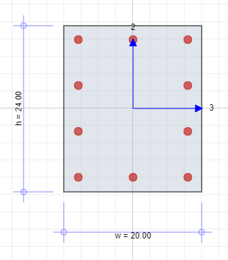
The moment magnification calculation for a given rectangular section using ACI 318-19 is tested in this example by comparing the results with manual calculation.
The column section details are as tabulated below.
Note: Refer ACI 318-19 Moment Magnification Sway Ex001.cdbx
|
Parameters | Value |
|---|---|---|
| Width (in) | 20 | |
| Height (in) | 24 | |
| Compressive Strength, fc’ (psi) | 4,000 | |
| Modulus of Elasticity of Concrete, Ec (ksi) | 3,600 | |
| Minimum Yield Stress, fy (psi) | 40,000 | |
| Modulus of Elasticity of Steel, Es (ksi) | 29,000 | |
| Rebar Layout | 10-#9 | |
| Rebar Area (in2) | 9.99 | |
| Rebar Ratio | 2.08% | |
| Clear Cover (in) | 1.5 | |
| C/C Length, lc (ft) | 17.5 | |
| Unsupported Length, lu (ft) | 17 | |
| k-factor, Unbraced (YZ Plane) | 1.5 | |
| k-factor, Braced (YZ Plane) | 0.78 |
| Name | Non-Sway Part | Sway Part | |||||
|---|---|---|---|---|---|---|---|
| Axial Load, Pu (kip) | Moment Top, Mux (kip-ft) |
Moment Bottom, Mux (kip-ft) |
Sustained Load (kip) |
Axial Load, Pu (kip) | Moment Top, Mux (kip-ft) |
Moment Bottom, Mux (kip-ft) |
|
| Combo1 | 350 | 48 | -55 | 250 | 10 | 76 | -72 |
| Parameter | Value |
|---|---|
| Story Axial Load, ∑Pu (kip) | 12,000 |
| Story Critical Load, ∑Pc (kip) | 40,000 |
| Relative Sway, Δ (in) | 0.3 |
| Story Shear Load, Vus (kip) | 243 |
MOMENT MAGNIFICATION COMPARISON
Column Designer reports both the top and bottom magnified moments in X and Y direction. The higher of the top and bottom magnified moments is reported as M2 while the lower magnified moment is reported as M1.
| Magnified Moments (kip-ft) | Column Designer | By hand | % Difference |
|---|---|---|---|
| M1x | 129.77 | 129.77 | 0.00% |
| M2x | -132.46 | -132.46 | 0.00% |
MANUAL CALCULATION
| Calculation of Magnified Moment about X-axis | ||||||
|---|---|---|---|---|---|---|
| Loading Data | ||||||
| M1ns | = | 576 | kip-in | |||
| M2ns | = | -660 | kip-in | |||
| Axial Load, Non-sway Part (Pu) | = | 350 | kip | |||
| M1s | = | 912 | kip-in | |||
| M2s | = | -864 | kip-in | |||
| Axial Load, Sway Part (Pu) | = | 10 | kip | |||
| Calculation of δs | ||||||
| ΣPu | = | 12,000 | kip | |||
| ΣPc | = | 40,000 | kip | |||
| Relative Lateral Deflection, Δo | = | 0.3 | in | |||
| Story Shear, Vus | = | 243 | kip | |||
| C/C length of Column, lc | = | 210 | in | |||
| Q | = | \[\frac{\sum_{}^{}{P_{u}\mathrm{\Delta}_{o}}}{V_{us}l_{c}}\] | [ACI 318-19 6.6.4.4.1] | |||
| = | 0.07 | |||||
| δs | = | \[\frac{1}{1 - Q}\] | ≥ 1 | [ACI 318-19 6.6.4.6.2a] | ||
| = | 1.08 | |||||
| Calculation of M1 and M2 | ||||||
| M1 (Lower Moment) | = | M1ns + δsM1s | [ACI 318-19 6.6.4.6.1a] | |||
| = | 1557.22 | kip-in | ||||
| M2 (Higher Moment) | = | M2ns + δsM2s | [ACI 318-19 6.6.4.6.1b] | |||
| = | -1589.58 | kip-in | ||||
| Magnification along Column Length | ||||||
| Calculation of Critical Buckling Load | ||||||
| K factor (Braced) | = | 0.78 | ||||
| Unsupported Length, lu | = | 204 | in | |||
| (Ig)column | = | \[\frac{20*24^{3}}{12}\] | in4 | |||
| = | 23,040 | in4 | ||||
| Ec | = | 3,600 | ksi | |||
| 0.2EcIg | = | 16,588,800 | kip-in2 | |||
| Es | = | 29,000 | ksi | |||
| Ise | = | 636.59 | in4 | |||
| βdns | = | 0.69 | ||||
| (EI)eff | = | \[\frac{0.2E_{c}I_{g} + E_{s}I_{se}}{1 + \beta_{dns}}\] | kip-in2 | [ACI 318-19 6.6.4.4.4] | ||
| = | 20,685,178.28 | kip-in2 | ||||
| Critical Buckling Load, Pc | = | \[\frac{\pi^{2}{(EI)}_{eff}}{{(kl_{u})}^{2}}\] | kip | [ACI 318-19 6.6.4.4.2] | ||
| = | 8,063.24 | kip | ||||
| Calculation of Cm | ||||||
| Cm | = | \[0.6 - 0.4\frac{M_{1}}{M_{2}}\] | ≥0.4 |
\[\lbrack\frac{M_{1}}{M_{2}} = + ve\ for\ double\ curvature\rbrack\] [ACI 318-19 6.6.4.5.3] |
||
| = | 0.4 | |||||
| Calculation of Magnification Factor | ||||||
| δ | = | \[\frac{C_{m}}{1 - \frac{P_{u}}{0.75P_{c}}}\] | ≥ 1 | [ACI 318-19 6.6.4.5.2] | ||
| = | 1 | |||||
| Calculation of Final Magnified Moments | ||||||
| M1 | = | 1,557.22 | kip-in | |||
| = | 129.77 | kip ft | ||||
| M2 | = | -1,589.58 | kip-in | |||
| = | -132.46 | kip ft | ||||
ACI 318-19 Moment Magnification Sway- Example 002
Moment Magnification Calculation for Slender Column (Sway)
GEOMETRY, PROPERTIES AND LOADING
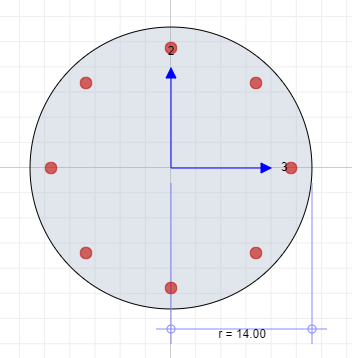
The moment magnification calculation for a given circular section using ACI 318-19 is tested in this example by comparing the results with manual calculation.
The column section details are as tabulated below.
Note: Refer ACI 318-19 Moment Magnification Sway Ex002.cdbx
|
Parameters | Value |
|---|---|---|
| Diameter (in) | 28 | |
| Compressive Strength, fc’ (psi) | 4,000 | |
| Modulus of Elasticity of Concrete, Ec (ksi) | 3,600 | |
| Minimum Yield Stress, fy (psi) | 40,000 | |
| Modulus of Elasticity of Steel, Es (ksi) | 29,000 | |
| Rebar Layout | 8-#9 | |
| Rebar Area (in2) | 7.99 | |
| Rebar Ratio | 1.30% | |
| Clear Cover (in) | 1.5 | |
| C/C Length, lc (ft) | 17.5 | |
| Unsupported Length, lu (ft) | 17 | |
| k-factor, Unbraced (YZ Plane) | 1.51 | |
| k-factor, Braced (YZ Plane) | 0.81 |
| Name | Non-Sway Part | Sway Part | |||||
|---|---|---|---|---|---|---|---|
| Axial Load, Pu (kip) | Moment Top, Mux (kip-ft) |
Moment Bottom, Mux (kip-ft) |
Sustained Load (kip) |
Axial Load, Pu (kip) | Moment Top, Mux (kip-ft) |
Moment Bottom, Mux (kip-ft) |
|
| Combo1 | 500 | 125 | 135 | 342 | 13 | 92 | 108 |
| Parameter | Value |
|---|---|
| Story Axial Load, ∑Pu (kip) | 25,000 |
| Story Critical Load, ∑Pc (kip) | 83,333 |
| Relative Sway, Δ (in) | 0.24 |
| Story Shear Load, Vus (kip) | 316 |
MOMENT MAGNIFICATION COMPARISON
Column Designer reports both the top and bottom magnified moments in X and Y direction. The higher of the top and bottom magnified moments is reported as M2 while the lower magnified moment is reported as M1.
| Magnified Moments (kip-ft) | Column Designer | By hand | % Difference |
|---|---|---|---|
| M1x | 235.75 | 235.74 | 0.01% |
| M2x | 264.52 | 264.50 | 0.01% |
MANUAL CALCULATION
| Calculation of Magnified Moment about X-axis | ||||
|---|---|---|---|---|
| Loading Data | ||||
| M1ns | = | 1,500 | kip-in | |
| M2ns | = | 1,620 | kip-in | |
| Axial Load, Non-sway Part (Pu) | = | 500 | kip | |
| M1s | = | 1,104 | kip-in | |
| M2s | = | 1296 | kip-in | |
| Axial Load, Sway Part (Pu) | = | 13 | kip | |
| Calculation of δs | ||||
| ΣPu | = | 25,000 | kip | |
| ΣPc | = | 83,333 | kip | |
| Relative Lateral Deflection, Δo | = | 0.24 | in | |
| Story Shear, Vus | = | 316 | kip | |
| C/C length of Column, lc | = | 210 | in | |
| Q | = | \[\frac{\sum_{}^{}{P_{u}\mathrm{\Delta}_{o}}}{V_{us}l_{c}}\] | [ACI 318-19 6.6.4.4.1] | |
| = | 0.09 | |||
| δs | = | \[\frac{1}{1 - Q}\] | ≥ 1 | [ACI 318-19 6.6.4.6.2a] |
| = | 1.10 | |||
| Calculation of M1 and M2 | ||||
| M1 (Lower Moment) | = | M1ns + δsM1s | [ACI 318-19 6.6.4.6.1a] | |
| = | 2713.74 | kip-in | ||
| M2 (Higher Moment) | = | M2ns + δsM2s | [ACI 318-19 6.6.4.6.1b] | |
| = | 3,044.83 | kip-in | ||
| Magnification along Column Length | ||||
| Calculation of Critical Buckling Load | ||||
| K factor (Braced) | = | 0.81 | ||
| Unsupported Length, lu | = | 204 | in | |
| (Ig)column | = | \[\frac{\pi*14^{4}}{4}\] | in4 | |
| = | 30,171.86 | in4 | ||
| Ec | = | 3600 | ksi | |
| 0.2EcIg | = | 21,723,736.21 | kip-in2 | |
| Es | = | 29,000 | ksi | |
| Ise | = | 570.13 | in4 | |
| βdns | = | 0.67 | ||
| (EI)eff | = | \[\frac{0.2E_{c}I_{g} + E_{s}I_{se}}{1 + \beta_{dns}}\] | kip-in2 | [ACI 318-19 6.6.4.4.4] |
| = | 22,954,420.67 | kip-in2 | ||
| Critical Buckling Load, Pc | = | \[\frac{\pi^{2}{(EI)}_{eff}}{{(kl_{u})}^{2}}\] | kip | [ACI 318-19 6.6.4.4.2] |
| = | 8,297.28 | kip | ||
| Calculation of Cm | ||||
| Cm | = | \[0.6 - 0.4\frac{M_{1}}{M_{2}}\] | ≥0.4 |
\[\lbrack\frac{M_{1}}{M_{2}} = - ve\ for\ single\ curvature\rbrack\] [ACI 318-19 6.6.4.5.3] |
| = | 0.96 | |||
| Calculation of Magnification Factor | ||||
| δ | = | \[\frac{C_{m}}{1 - \frac{P_{u}}{0.75P_{c}}}\] | ≥ 1 | [ACI 318-19 6.6.4.5.2] |
| = | 1.04 | |||
| Calculation of Final Magnified Moments | ||||
| M1 | = | 2,828.91 | kip-in | |
| = | 235.74 | kip ft | ||
| M2 | = | 3,174.05 | kip-in | |
| = | 264.50 | kip ft | ||
Eurocode 2-2004 Moment Magnification Sway- Example 001
Moment Magnification Calculation for Slender Column (Sway)
GEOMETRY, PROPERTIES AND LOADING
The moment magnification calculation for a given rectangular section using Eurocode 2:2004 is tested in this example by comparing the results with manual calculation.
The column section details are as tabulated below.
Note: Refer Eurocode 2-2004 Moment Magnification Sway Ex001.cdbx
|
|
Parameters | Value |
|---|---|---|
| Width, w (mm) | 400 | |
| Height, h (mm) | 500 | |
| Rebar Layout | 12-d25 | |
| Clear Cover, cc (mm) | 40 | |
| Compressive Strength, fck (MPa) | 40 | |
| Minimum Yield Stress, fyk (MPa) | 500 | |
| Modulus of Elasticity of Concrete, Ec (MPa) | 35,000 | |
| Modulus of Elasticity of Steel, Es (MPa) | 200,000 | |
| Concrete Area, Ac (mm2) | 200,000 | |
| Rebar Area, As (mm2) | 5,890.49 | |
| Concrete Inertia, Ig, 22 (mm4) | 2.667x10⁹ | |
| Concrete Inertia, Ig, 33 (mm4) | 4.167x10⁹ | |
| Rebar Inertia, Is, 22 (mm4) | 9.018 x10⁷ | |
| Rebar Inertia, Is, 33 (mm4) | 1.617x10⁸ | |
| Perimeter, u (mm) | 1,800 | |
| Relative Humidity, RH (%) | 50 | |
| Ratio SLS to ULS moments, rm | 0.8 | |
| Age of concrete at loading, t0 (days) | 28 | |
| Concrete partial safety factor, γc | 1.5 | |
| Reinforcing partial safety factor, γs | 1.15 | |
| Long term compressive strength factor, αcc | 1 | |
| Unsupported Length, lu (m) | 3 | |
| Effective Length Factor (Unbraced), kXZ | 2.94 | |
| Effective Length Factor (Unbraced), kYZ | 4.26 | |
| Biaxial Loading | Yes |
| Name | Axial Load, NEd (kN) |
Moment Top, Mx,top (kN-m) |
Moment Top, My,top (kN-m) |
Moment Bottom, Mx,bot (kN-m) |
Moment Bottom, My,bot (kN-m) |
|---|---|---|---|---|---|
| Combination 1 | 1000 | 110 | 250 | 120 | 210 |
MOMENT MAGNIFICATION COMPARISON
Column Designer reports both the design moments in X and Y direction. The design moments are reported as the top moments for capacity calculations, while the bottom moments remain unchanged.
| Design Moments (kN-m) | Column Designer | By hand | % Difference |
|---|---|---|---|
| \(M_{Ed,x}\) | 337.77 | 337.74 | 0.01% |
| \(M_{Ed,y}\) | 379.13 | 379.12 | 0.01% |
| \(M_{c}\) | 603.23 | 603.20 | 0.01% |
MANUAL CALCULATION
| Calculation of Design Moment about X-axis | |||||
|---|---|---|---|---|---|
| Loading Data | |||||
| Moment Top, Mx, top | = | 110,000,000 | N-mm | ||
| Moment Bottom, Mx, bot | = | 120,000,000 | N-mm | ||
| Axial Load, NEd | = | 1,000,000 | N | ||
| Calculation of Additional Parameters | |||||
| Effective Length, l0 | = | kYZ × lu | [EC2 5.8.3.2 (3)] | ||
| = | 4.26×3,000 | ||||
| = | 12780 | mm | |||
| Design Compressive Strength, fcd | = | \[\alpha_{cc} \times \frac{f_{ck}}{\gamma_{c}}\] | [EC2 3.1.6 (1)] | ||
| = | 1×40/1.5 | ||||
| = | 26.67 | MPa | |||
| Mean Value Cylinder Compressive Strength, fcm | = | fck + 8 | [EC2 Table 3.1] | ||
| = | 40+8 | ||||
| = | 48 | MPa | |||
| Design Yield Strength, fyd | = | \[\frac{f_{yk}}{\gamma_{s}}\] | [EC2 3.2.7 (2)] | ||
| = | 500⁄1.15 | ||||
| = | 434.78 | MPa | |||
| Design Strain, εyd | = | \[\frac{f_{yd}}{E_{s}}\] | [EC2 5.8.8.3 (1)] | ||
| = | 434.78/200,000 | ||||
| = | 0.002174 | mm/mm | |||
| Curvature Distribution Factor, c | = | 10 | [EC2 5.8.8.2 (4)] | ||
| Radius of Gyration of Concrete Section, rc | = | \[\sqrt{\frac{I_{g,33}}{A_{c}}}\] | |||
| = | \[\sqrt{\frac{4.167 \times 10^{9}}{200,000}}\] | ||||
| = | 144.34 | mm | |||
| Radius of Gyration of Rebar, rs | = | \[\sqrt{\frac{I_{s,33}}{A_{s}}}\] | |||
| = | \[\sqrt{\frac{1.617 \times 10^{8}}{5,890.49}}\] | ||||
| = | 165.68 | mm | |||
| Effective Depth, d | = | \[\frac{h}{2} + r_{s}\] | [EC2 5.8.8.3 (2)] | ||
| = | 500/2+165.68 | ||||
| = | 415.68 | mm | |||
| Determine First Order End Moments | |||||
| Determine M01 and M02 to satisfy |M02| ≥ |M01| | [EC2 5.8.8.2 (2)] | ||||
|
NOTE:
|
[IStructE Manual EC2 5.5.4.2] | ||||
| Lower End Moment, M01 | = | min {Mx, top, Mx, bot} | |||
| = | 110,000,000 | N-mm | |||
| Higher End Moment, M02 | = | max {Mx, top, Mx, bot} | |||
| = | 120,000,000 | N-mm | |||
| Calculate Curvature | |||||
| Mechanical Reinforcement Ratio, ω | = | \[\frac{A_{s} \times f_{yd}}{A_{c} \times f_{cd}}\\] | [EC2 5.8.8.3 (3)] | ||
| = | (5,890.49×434.78)/ (200,000×26.67) | ||||
| = | 0.4801 | ||||
| Relative Ultimate Axial Load, nu | = | 1 + ω | [EC2 5.8.8.3 (3)] | ||
| = | 1+0.4801 | ||||
| = | 1.4801 | ||||
| Relative Axial Force, n | = | \[\frac{N_{Ed}}{\left( A_{c} \times f_{cd} \right)}\] | [EC2 5.8.8.3 (3)] | ||
| = | 1,000,000/ (200,000×26.67) | ||||
| = | 0.1875 | ||||
| Relative Balanced Load, nbal | = | 0.4 | [EC2 5.8.8.3 (3)] | ||
| Axial Load Correction Factor, Kr | = | \[\frac{nu - n}{nu - n_{bal}} \leq 1\] | [EC2 5.8.8.3 (3)] | ||
| = | \[\frac{1.4801 - 0.4}{1.4801 - 0.1875} \leq 1\] | ||||
| = | 1 | ||||
| Member Notional Size, h0 | = | \[\frac{2 \times A_{c}}{u}\] | [EC2 Annex B.1 (1) Eqn(B.6)] | ||
| = | (2×200,000)/1800 | ||||
| = | 222.22 | mm | |||
| Influence of Concrete Strength Coefficient, α1 | = | \[\left( \frac{35}{f_{cm}} \right)^{0.7}\] | [EC2 Annex B.1 (1) Eqn(B.8c)] | ||
| = | (35⁄48)0.7 | ||||
| = | 0.8016 | ||||
| Influence of Concrete Strength Coefficient, α2 | = | \[\left( \frac{35}{f_{cm}} \right)^{0.2}\] | [EC2 Annex B.1 (1) Eqn(B.8c)] | ||
| = | (35⁄48)0.2 | ||||
| = | 0.9388 | ||||
| Factor for Effect of Relative Humidity on Notional Creep Coefficient, φRH | [EC2 Annex B.1 (1) Eqn(B.3)] | ||||
|
NOTE:
|
|||||
| φRH | = | \[\left\lbrack 1 + \left( \frac{1 - \frac{RH}{100}}{0.1 \times \sqrt[3]{h_{0}}} \times \alpha_{1} \right) \right\rbrack \times \alpha_{2}\] | |||
| = | \[\left\lbrack 1 + \left( \frac{1 - \frac{50}{100}}{0.1 \times \sqrt[3]{222.22}} \times 0.8016 \right) \right\rbrack \times 0.9388\] | ||||
| = | 1.56 | ||||
| Factor for Effect of Concrete Strength on Notional Creep Coefficient, β(fcm) | = | \[\frac{16.8}{\sqrt{f_{cm}}}\] | [EC2 Annex B.1 (1) Eqn(B.4)] | ||
| = | \[\frac{16.8}{\sqrt{48}}\] | ||||
| = | 2.425 | ||||
| Factor for Effect of Concrete Age on Notional Creep Coefficient, β(t0) | = | \[\frac{1}{\left( 0.1 + {t_{0}}^{0.2} \right)}\] | [EC2 Annex B.1 (1) Eqn(B.5)] | ||
| = | \[\frac{1}{\left( 0.1 + 28^{0.2} \right)}\] | ||||
| = | 0.4884 | ||||
| Notional Creep Coefficient, φ0 | = | φRH × β(fcm) × β(t0) | [EC2 Annex B.1 (1) Eqn(B.2)] | ||
| = | 1.56×2.425×0.4884 | ||||
| = | 1.848 | ||||
| Effective Creep Ratio, φef | = | φ0 × rm | [EC2 5.8.4 (2)] | ||
| = | 1.848×0.8 | ||||
| = | 1.4784 | ||||
| Slenderness Ratio, λ | = | \[\frac{l_{0}}{r}_{c}\] | [EC2 5.8.3.2 (1)] | ||
| = | 12780/144.34 | ||||
| = | 88.54 | ||||
| Factor, β | = | \[0.35 + \frac{f_{ck}}{200} - \frac{\lambda}{150}\] | [EC2 5.8.8.3 (4)] | ||
| = | 0.35+40/200-88.54/150 | ||||
| = | -0.0403 | ||||
| Creep Factor, Kφ | = | 1 + β × φef ≥ 1 | [EC2 5.8.8.3 (4)] | ||
| = | 1 + (−0.0403) × 1.4784 ≥ 1 | ||||
| = | 1 | ||||
| Curvature, \(\frac{1}{r}\) | = | \[K_{r} \times K_{\varphi} \times \frac{\varepsilon_{yd}}{0.45d}\] | [EC2 5.8.8.3 (1)] | ||
| = | 1×1×0.002174⁄0.45(415.68) | ||||
| = | 0.00001162 | 1/mm | |||
| Calculate Moment due to Geometric Imperfections | |||||
| Eccentricity due to Geometric Imperfections, ei | = | \[\max\left\{ \frac{l_{0}}{400},\frac{h}{30},20 \right\}\] | [EC2 5.2 (7)a] | ||
| = | \[\max\left\{ \frac{12780}{400},\frac{500}{30},20 \right\}\] | [EC2 6.1 (4)] | |||
| = | 31.95 | mm | |||
| Geometric Imperfections Moment, Mi | = | NEd × ei | [EC2 5.2 (7) Fig 5.1a] | ||
| = | 1,000,000×31.95 | ||||
| = | 31,950,000 | N-mm | |||
| Calculate First Order Moment | |||||
| First Order Moment, M0e | = | 0.6M02 + 0.4M01 ≥ 0.4M02 | [EC2 5.8.8.2 (2)] | ||
| = | 0.6 × 120, 000, 000 + 0.4 × 110, 000, 000 ≥ 0.4 × 120, 000, 000 | ||||
| = | 116,000,000 | N-mm | |||
| Included Effect of Imperfections, M0Ed | = | M0e + Mi | [EC2 5.8.8.2 (1)] | ||
| = | 116,000,000+31,950,000 | ||||
| = | 147,950,000 | N-mm | |||
| Calculate Nominal Second Order Moment | |||||
| Deflection, e2 | = | \[\left( \frac{1}{r} \right) \times {l_{0}}^{2}/c\] | [EC2 5.8.8.2 (3)] | ||
| = | 0.00001162×127802/10 | ||||
| = | 189.79 | mm | |||
| Nominal Second Order Moment, M2 | = | NEd × e2 | [EC2 5.8.8.2 (3)] | ||
| = | 1,000,000×189.79 | ||||
| = | 189,790,000 | N-mm | |||
| Calculate Design Moment | |||||
| The design moment is the maximum of: | |||||
|
= | 120 | kN-m | [EC2 5.8.8.2 (1)] | |
|
= | 147.95+189.79 | [Concise EC2 5.6.2.2] | ||
| = | 337.74 | kN-m | |||
|
= | 110+0.5×189.79 | |||
| = | 204.90 | kN-m | |||
|
= | 1,000×max (400/30,20) | |||
| = | 20 | kN-m | |||
| Design Moment, MEd, x | = | \[\max\left\{ M_{02},M_{0Ed} + M_{2},M_{01} + 0.5M_{2},N_{Ed} \times \max\left( \frac{b}{30},20 \right) \right\}\] | |||
| = | 337.74 | kN-m | |||
| Calculation of Design Moment about Y-axis | ||||
|---|---|---|---|---|
| Loading Data | ||||
| Moment Top, My, top | = | 250,000,000 | N-mm | |
| Moment Bottom, My, bot | = | 210,000,000 | N-mm | |
| Axial Load, NEd | = | 1,000,000 | N | |
| Calculation of Additional Parameters | ||||
| Effective Length, l0 | = | kXZ × lu | [EC2 5.8.3.2 (3)] | |
| = | 2.94×,3000 | |||
| = | 8,820 | mm | ||
| Design Compressive Strength, fcd | = | \[\alpha_{cc} \times \frac{f_{ck}}{\gamma_{c}}\] | [EC2 3.1.6 (1)] | |
| = | 1×40⁄1.5 | |||
| = | 26.67 | MPa | ||
| Mean Value Cylinder Compressive Strength, fcm | = | fck + 8 | [EC2 Table 3.1] | |
| = | 40+8 | |||
| = | 48 | MPa | ||
| Design Yield Strength, fyd | = | \[\frac{f_{yk}}{\gamma_{s}}\] | [EC2 3.2.7 (2)] | |
| = | 500⁄1.15 | |||
| = | 434.78 | MPa | ||
| Design Strain, εyd | = | \[\frac{f_{yd}}{E_{s}}\] | [EC2 5.8.8.3 (1)] | |
| = | 434.78/200,000 | |||
| = | 0.002174 | mm/mm | ||
| Curvature Distribution Factor, c | = | 10 | [EC2 5.8.8.2 (4)] | |
| Radius of Gyration of Concrete Section, rc | = | \[\sqrt{\frac{I_{g,33}}{A_{c}}}\] | ||
| = | \[\sqrt{\frac{2.667 \times 10^{9}}{200,000}}\] | |||
| = | 115.48 | mm | ||
| Radius of Gyration of Rebar, rs | = | \[\sqrt{\frac{I_{s,33}}{A_{s}}}\] | ||
| = | \[\sqrt{\frac{9.018 \times 10^{7}}{5,890.49}}\] | |||
| = | 123.73 | mm | ||
| Effective Depth, d | = | \[\frac{w}{2} + r_{s}\] | [EC2 5.8.8.3 (2)] | |
| = | 400⁄2+123.73 | |||
| = | 323.73 | mm | ||
| Determine First Order End Moments | ||||
| Determine M01 and M02 to satisfy |M02| ≥ |M01| | [EC2 5.8.8.2 (2)] | |||
|
NOTE:
|
[IStructE Manual EC2 5.5.4.2] | |||
| Lower End Moment, M01 | = | min {My, top, My, bot} | ||
| = | 210,000,000 | N-mm | ||
| Higher End Moment, M02 | = | max {My, top, My, bot} | ||
| = | 250,000,000 | N-mm | ||
| Calculate Curvature | ||||
| Mechanical Reinforcement Ratio, ω | = | \[\frac{A_{s} \times f_{yd}}{A_{c} \times f_{cd}}\\] | [EC2 5.8.8.3 (3)] | |
| = | (5890.49×434.78)/ (200,000×26.67) | |||
| = | 0.4801 | |||
| Relative Ultimate Axial Load, nu | = | 1 + ω | [EC2 5.8.8.3 (3)] | |
| = | 1+0.4801 | |||
| = | 1.4801 | |||
| Relative Axial Force, n | = | \[\frac{N_{Ed}}{\left( A_{c} \times f_{cd} \right)}\] | [EC2 5.8.8.3 (3)] | |
| = | 1,000,000/ (200,000×26.67) | |||
| = | 0.1875 | |||
| Relative Balanced Load, nbal | = | 0.4 | [EC2 5.8.8.3 (3)] | |
| Axial Load Correction Factor, Kr | = | \[\frac{nu - n}{nu - n_{bal}} \leq 1\] | [EC2 5.8.8.3 (3)] | |
| = | \[\frac{1.4801 - 0.4}{1.4801 - 0.1875} \leq 1\] | |||
| = | 1 | |||
| Member Notional Size, h0 | = | \[\frac{2 \times A_{c}}{u}\] | [EC2 Annex B.1 (1) Eqn(B.6)] | |
| = | (2×200,000)/1800 | |||
| = | 222.22 | mm | ||
| Influence of Concrete Strength Coefficient, α1 | = | \[\left( \frac{35}{f_{cm}} \right)^{0.7}\] | [EC2 Annex B.1 (1) Eqn(B.8c)] | |
| = | \[\left( \frac{35}{48} \right)^{0.7}\] | |||
| = | 0.8016 | |||
| Influence of Concrete Strength Coefficient, α2 | = | \[\left( \frac{35}{f_{cm}} \right)^{0.2}\] | [EC2 Annex B.1 (1) Eqn(B.8c)] | |
| = | \[\left( \frac{35}{48} \right)^{0.2}\] | |||
| = | 0.9388 | |||
| Factor for Effect of Relative Humidity on Notional Creep Coefficient, φRH | [EC2 Annex B.1 (1) Eqn(B.3)] | |||
|
NOTE:
|
||||
| φRH | = | \[\left\lbrack 1 + \left( \frac{1 - \frac{RH}{100}}{0.1 \times \sqrt[3]{h_{0}}} \times \alpha_{1} \right) \right\rbrack \times \alpha_{2}\] | ||
| = | \[\left\lbrack 1 + \left( \frac{1 - \frac{50}{100}}{0.1 \times \sqrt[3]{222.22}} \times 0.8016 \right) \right\rbrack \times 0.9388\] | |||
| = | 1.56 | |||
| Factor for Effect of Concrete Strength on Notional Creep Coefficient, β(fcm) | = | \[\frac{16.8}{\sqrt{f_{cm}}}\] | [EC2 Annex B.1 (1) Eqn(B.4)] | |
| = | \[\frac{16.8}{\sqrt{48}}\] | |||
| = | 2.425 | |||
| Factor for Effect of Concrete Age on Notional Creep Coefficient, β(t0) | = | \[\frac{1}{\left( 0.1 + {t_{0}}^{0.2} \right)}\] | [EC2 Annex B.1 (1) Eqn(B.5)] | |
| = | \[\frac{1}{\left( 0.1 + 28^{0.2} \right)}\] | |||
| = | 0.4884 | |||
| Notional Creep Coefficient, φ0 | = | φRH × β(fcm) × β(t0) | [EC2 Annex B.1 (1) Eqn(B.2)] | |
| = | 1.56×2.425×0.4884 | |||
| = | 1.848 | |||
| Effective Creep Ratio, φef | = | φ0 × rm | [EC2 5.8.4 (2)] | |
| = | 1.848×0.8 | |||
| = | 1.4784 | |||
| Slenderness Ratio, λ | = | \[\frac{l_{0}}{r}_{c}\] | [EC2 5.8.3.2 (1)] | |
| = | 8,820⁄115.48 | |||
| = | 76.37 | |||
| Factor, β | = | \[0.35 + \frac{f_{ck}}{200} - \frac{\lambda}{150}\] | [EC2 5.8.8.3 (4)] | |
| = | 0.35+40/200-76.37/150 | |||
| = | 0.0409 | |||
| Creep Factor, Kφ | = | 1 + β × φef ≥ 1 | [EC2 5.8.8.3 (4)] | |
| = | 1 + 0.0409 × 1.4784 ≥ 1 | |||
| = | 1.060 | |||
| Curvature, \(\frac{1}{r}\) | = | \[K_{r} \times K_{\varphi} \times \frac{\varepsilon_{yd}}{0.45d}\] | [EC2 5.8.8.3 (1)] | |
| = | 1×1.060×0.002174/0.45(323.73) | |||
| = | 0.00001582 | 1/mm | ||
| Calculate Moment due to Geometric Imperfections | ||||
| Eccentricity due to Geometric Imperfections, ei | = | \[\max\left\{ \frac{l_{0}}{400},\frac{w}{30},20 \right\}\] | [EC2 5.2 (7)a] | |
| = | \[\max\left\{ \frac{8820}{400},\frac{400}{30},20 \right\}\] | [EC2 6.1 (4)] | ||
| = | 22.05 | mm | ||
| Geometric Imperfections Moment, Mi | = | NEd × ei | [EC2 5.2 (7) Fig 5.1a] | |
| = | 1000,000×22.05 | |||
| = | 22,050,000 | N-mm | ||
| Calculate First Order Moment | ||||
| First Order Moment, M0e | = | 0.6M02 + 0.4M01 ≥ 0.4M02 | [EC2 5.8.8.2 (2)] | |
| = | 0.6 × 250, 000, 000 + 0.4 × 210, 000, 000 ≥ 0.4 × 250, 000, 000 | |||
| = | 234,000,000 | N-mm | ||
| Included Effect of Imperfections, M0Ed | = | M0e + Mi | [EC2 5.8.8.2 (1)] | |
| = | 234,000,000+22,050,000 | |||
| = | 256,050,000 | N-mm | ||
| Calculate Nominal Second Order Moment | ||||
| Deflection, e2 | = | \[\left( \frac{1}{r} \right) \times {l_{0}}^{2}/c\] | [EC2 5.8.8.2 (3)] | |
| = | 0.00001582×8,8202/10 | |||
| = | 123.07 | mm | ||
| Nominal Second Order Moment, M2 | = | NEd × e2 | [EC2 5.8.8.2 (3)] | |
| = | 1,000,000×123.07 | |||
| = | 123,070,000 | N-mm | ||
| Calculate Design Moment | ||||
| The design moment is the maximum of: | ||||
|
= | 250 | kN-m | [EC2 5.8.8.2 (1)] |
|
= | 256.05+123.07 | [Concise EC2 5.6.2.2] | |
| = | 379.12 | kN-m | ||
|
= | 210+0.5×123.07 | ||
| = | 271.54 | kN-m | ||
|
= | 1000×max (500/30,20) | ||
| = | 20 | kN-m | ||
| Design Moment, MEd, y | = | \[\max\left\{ M_{02},M_{0Ed} + M_{2},M_{01} + 0.5M_{2},N_{Ed} \times \max\left( \frac{b}{30},20 \right) \right\}\] | ||
| = | 379.12 | kN-m | ||
| Increased Design Moment due to Biaxial Bending | ||||
|---|---|---|---|---|
| Calculate Effective Depths | [IStructE Manual EC2 5.5.5] | |||
| Effective Height, h′ | = | \[\max\left\{ h - c_{c} - \frac{c_{b}}{2},w - c_{c} - \frac{c_{b}}{2} \right\}\] | ||
| = | \[\max\left\{ 500 - 40 - \frac{25}{2},400 - 40 - \frac{25}{2} \right\}\] | |||
| = | 447.5 | mm | ||
| Effective Width, b′ | = | \[\min\left\{ h - c_{c} - \frac{c_{b}}{2},w - c_{c} - \frac{c_{b}}{2} \right\}\] | ||
| = | \[\min\left\{ 500 - 40 - \frac{25}{2},400 - 40 - \frac{25}{2} \right\}\] | |||
| = | 347.5 | mm | ||
| Calculate Coefficient for Biaxial Bending | [IStructE Manual EC2 5.5.5] | |||
| β | = | \[1 - 1.165 \times min\left\{ 0.6,\ \frac{N_{Ed}}{\left( A_{c} \times f_{ck} \right)} \right\}\] | ||
| = | \[1 - 1.165 \times min\left\{ 0.6,\ \frac{1000000}{(200000 \times 40)} \right\}\] | |||
| = | 0.8544 | |||
| Calculate Increased Design Moment | [IStructE Manual EC2 5.5.5] | |||
|
NOTE:
|
||||
| Final Design Moment, Mc | = | \[M_{Ed,y} + \beta \times \frac{b'}{h'} \times M_{Ed,x}\\] | ||
| = | \[379.12 + 0.8544 \times \frac{347.5}{447.5} \times 337.74\\] | |||
| = | 603.20 | MPa | ||
BS 8110-97 Moment Magnification Sway- Example 001
Moment Magnification Calculation for Slender Column (Sway)
GEOMETRY, PROPERTIES AND LOADING
The moment magnification calculation for a given rectangular section using BS 8110-97 is tested in this example by comparing the results with manual calculation.
The column section details are as tabulated below.
Note: Refer BS 8110-97 Moment Magnification Sway Ex001.cdbx
|
|
Parameters | Value |
|---|---|---|
| Width, w (mm) | 400 | |
| Height, h (mm) | 500 | |
| Rebar Layout | 12-d25 | |
| Clear Cover, cc (mm) | 40 | |
| Compressive Strength, fcu (MPa) | 40 | |
| Minimum Yield Stress, fy (MPa) | 500 | |
| Concrete Area, Ac (mm2) | 200,000 | |
| Rebar Area, Asc (mm2) | 5,890.49 | |
| Unsupported Length, lu (m) | 3 | |
| Effective Length Factor (Unbraced), βXZ | 1.99 | |
| Effective Length Factor (Unbraced), βYZ | 3.23 | |
| Biaxial Loading | Yes |
| Name |
Axial Load, N (kN) |
Moment Top, Mx,top (kN-m) |
Moment Top, My,top (kN-m) |
Moment Bottom, Mx,bot (kN-m) |
Moment Bottom, My,bot (kN-m) |
|---|---|---|---|---|---|
| Combination 1 | 1,000 | 110 | 250 | 120 | 210 |
MOMENT MAGNIFICATION COMPARISON
Column Designer reports both the design moments in X and Y direction. The design moments are reported as the top moments for capacity calculations, while the bottom moments remain unchanged.
| Design Moments (kN-m) | Column Designer | By hand | % Difference |
|---|---|---|---|
| \(M_{x}\) | 204.79 | 209.90 | 2.43% |
| \(M_{y}\) | 276.13 | 278.56 | 0.01% |
| \(M_{c}\) | 412 | 417.82 | 0.87% |
MANUAL CALCULATION
| Calculation of Design Moment about X-axis | ||||
|---|---|---|---|---|
| Loading Data | ||||
| Moment Top, Mx, top | = | 110,000,000 | N-mm | |
| Moment Bottom, Mx, bot | = | 120,000,000 | N-mm | |
| Axial Load, N | = | 1,000,000 | N | |
| Calculation of Additional Parameters | ||||
| Effective Length, le | = | βYZ × lu | [BS 8110-1 3.8.1.6.1] | |
| = | 3.23×3,000 | |||
| = | 9690 | mm | ||
| Balanced Section Axial Load, Nbal | = | 0.25 × fcu × Ac | [BS 8110-1 3.8.1.1] | |
| = | 0.25×40×200,000 | |||
| = | 2000,000 | N | ||
| Determine First Order End Moments | ||||
| Determine M1 and M2 to satisfy |M2| ≥ |M1| | [BS 8110-1 3.8.3.2] | |||
|
NOTE:
|
||||
| Lower End Moment, M1 | = | min {Mx, top, Mx, bot} | ||
| = | 110,000,000 | N-mm | ||
| Higher End Moment, M2 | = | max {Mx, top, Mx, bot} | ||
| = | 120,000,000 | N-mm | ||
| Calculate Additional Moment | ||||
| Section Ultimate Capacity to Axial Load, Nuz | = | 0.45 × fcu × Ac + 0.95 × fy × Asc | [BS 8110-1 3.8.3.1] | |
| = | 0.45×40×200000+0.95×500×5890.49 | |||
| = | 6,397,982.75 | N | ||
| Reduction Factor, K | = | \[\frac{N_{uz} - N}{N_{uz} - N_{bal}} \leq 1\] | [BS 8110-1 3.8.3.1] | |
| = | \[\frac{6,397,982.75\ - 1,000,000}{6,397,982.75\ - 2,000,000} \leq 1\] | |||
| = | 1 | |||
| Slenderness Factor, βa | [BS 8110-1 3.8.3.1] | |||
|
NOTE:
|
[BS 8110-1 3.8.3.6] | |||
| βa | = | \[\beta_{a} = \frac{1}{2,000}\left( \frac{l_{e}}{h} \right)^{2}\] | ||
| = | \[\beta_{a} = \frac{1}{2,000}\left( \frac{9,690}{500} \right)^{2}\] | |||
| = | 0.1878 | |||
| Deflection, au | = | βa × K × h | [BS 8110-1 3.8.3.1] | |
| = | 0.1878×1×500 | |||
| = | 93.9 | mm | ||
| Additional Moment, Madd | = | N × au | [BS 8110-1 3.8.3.1] | |
| = | 1,000,000×93.9 | |||
| = | 93,900,000 | N-mm | ||
| Calculate Initial Moment | ||||
| Initial Moment, Mi | = | 0.4M1 + 0.6M2 ≥ 0.4M2 | [BS 8110-1 3.8.3.2] | |
| = | 0.4 × 110, 000, 000 + 0.6 × 120, 000, 000 ≥ 0.4 × 120, 000, 000 | |||
| = | 116,000,000 | N-mm | ||
| Calculate Design Moment | ||||
| The design moment is the maximum of: | ||||
|
= | 120 | kN-m | [BS 8110-1 3.8.3.2] |
|
= | 116+93.9 | ||
| = | 209.9 | kN-m | ||
|
= | 110+0.5×93.9 | ||
| = | 156.95 | kN-m | ||
|
= | 1,000×max (0.05×500,20) | ||
| = | 25 | kN-m | ||
| Design Moment, Mx | = | max {M2, Mi + Madd, M1 + 0.5Madd, N × min (0.05 × h, 20)} | ||
| = | 209.9 | kN-m | ||
| Calculation of Design Moment about Y-axis | ||||
|---|---|---|---|---|
| Loading Data | ||||
| Moment Top, My, top | = | 250,000,000 | N-mm | |
| Moment Bottom, My, bot | = | 210,000,000 | N-mm | |
| Axial Load, N | = | 1,000,000 | N | |
| Calculation of Additional Parameters | ||||
| Effective Length, le | = | βXZ × lu | [BS 8110-1 3.8.1.6.1] | |
| = | 1.99×3,000 | |||
| = | 5,970 | mm | ||
| Balanced Section Axial Load, Nbal | = | 0.25 × fcu × Ac | [BS 8110-1 3.8.1.1] | |
| = | 0.25×40×200,000 | |||
| = | 2000,000 | N | ||
| Determine First Order End Moments | ||||
| Determine M1 and M2 to satisfy |M2| ≥ |M1| | [BS 8110-1 3.8.3.2] | |||
|
NOTE:
|
||||
| Lower End Moment, M1 | = | min {My, top, My, bot} | ||
| = | 210,000,000 | N-mm | ||
| Higher End Moment, M2 | = | max {My, top, My, bot} | ||
| = | 250,000,000 | N-mm | ||
| Calculate Additional Moment | ||||
| Section Ultimate Capacity to Axial Load, Nuz | = | 0.45 × fcu × Ac + 0.95 × fy × Asc | [BS 8110-1 3.8.3.1] | |
| = | 0.45×40×200,000+0.95×500×5890.49 | |||
| = | 6397982.75 | N | ||
| Reduction Factor, K | = | \[\frac{N_{uz} - N}{N_{uz} - N_{bal}} \leq 1\] | [BS 8110-1 3.8.3.1] | |
| = | \[\frac{6,397,982.75\ - 1,000,000}{6,397,982.75\ - 2,000,000} \leq 1\] | |||
| = | 1 | |||
| Slenderness Factor, βa | [BS 8110-1 3.8.3.1] | |||
|
NOTE:
|
[BS 8110-1 3.8.3.6] | |||
| βa | = | \[\beta_{a} = \frac{1}{2000}\left( \frac{l_{e}}{w} \right)^{2}\] | ||
| = | \[\beta_{a} = \frac{1}{2,000}\left( \frac{5970}{400} \right)^{2}\] | |||
| = | 0.1114 | |||
| Deflection, au | = | βa × K × w | [BS 8110-1 3.8.3.1] | |
| = | 0.1114×1×400 | |||
| = | 44.56 | mm | ||
| Additional Moment, Madd | = | N × au | [BS 8110-1 3.8.3.1] | |
| = | 1,000,000×44.56 | |||
| = | 44,560,000 | N-mm | ||
| Calculate Initial Moment | ||||
| Initial Moment, Mi | = | 0.4M1 + 0.6M2 ≥ 0.4M2 | [BS 8110-1 3.8.3.2] | |
| = | 0.4 × 21, 000, 0000 + 0.6 × 250, 000, 000 ≥ 0.4 × 250, 000, 000 | |||
| = | 234,000,000 | N-mm | ||
| Calculate Design Moment | ||||
| The design moment is the maximum of: | ||||
|
= | 250 | kN-m | [BS 8110-1 3.8.3.2] |
|
= | 234+44.56 | ||
| = | 278.56 | kN-m | ||
|
= | 210+0.5×44.56 | ||
| = | 232.28 | kN-m | ||
|
= | 1,000×max (0.05×400,20) | ||
| = | 20 | kN-m | ||
| Design Moment, My | = | max {M2, Mi + Madd, M1 + 0.5Madd, N × min (0.05 × w, 20)} | ||
| = | 278.56 | kN-m | ||
| Increased Design Moment due to Biaxial Bending | ||||
|---|---|---|---|---|
| Calculate Effective Depths | [BS 8110-1 3.8.4.5] | |||
| Effective Height, h′ | = | \[\max\left\{ h - c_{c} - \frac{c_{b}}{2},w - c_{c} - \frac{c_{b}}{2} \right\}\] | ||
| = | \[\max\left\{ 500 - 40 - \frac{25}{2},400 - 40 - \frac{25}{2} \right\}\] | |||
| = | 447.5 | mm | ||
| Effective Width, b′ | = | \[\min\left\{ h - c_{c} - \frac{c_{b}}{2},w - c_{c} - \frac{c_{b}}{2} \right\}\] | ||
| = | \[\min\left\{ 500 - 40 - \frac{25}{2},400 - 40 - \frac{25}{2} \right\}\] | |||
| = | 347.5 | mm | ||
| Calculate Coefficient for Biaxial Bending | [BS 8110-1 3.8.4.5] | |||
| β | = | \[1 - 1.165 \times min\left\{ 0.6,\ \frac{N}{\left( A_{c} \times f_{cu} \right)} \right\}\] | ||
| = | \[1 - 1.165 \times min\left\{ 0.6,\ \frac{1,000,000}{(200,000 \times 40)} \right\}\] | |||
| = | 0.8544 | |||
| Calculate Increased Design Moment | [BS 8110-1 3.8.4.5] | |||
|
NOTE:
|
||||
| Final Design Moment, Mc | = | \[M_{y} + \beta \times \frac{b'}{h'} \times M_{x}\\] | ||
| = | \[278.56 + 0.8544 \times \frac{347.5}{447.5} \times 209.9\\] | |||
| = | 417.82 | MPa | ||
IS 456-2000 Moment Magnification Sway- Example 001
Moment Magnification Calculation for Slender Column (Sway)
GEOMETRY, PROPERTIES AND LOADING
The moment magnification calculation for a given rectangular section using IS 456:2000 is tested in this example by comparing the results with manual calculation.
The column section details are as tabulated below.
Note: Refer IS 456-2000 Moment Magnification Sway Ex001.cdbx
|
|
Parameters | Value |
|---|---|---|
| Width, w (mm) | 400 | |
| Height, h (mm) | 500 | |
| Rebar Layout | 12-d25 | |
| Clear Cover, cc (mm) | 40 | |
| Compressive Strength, fck (MPa) | 40 | |
| Minimum Yield Stress, fy (MPa) | 500 | |
| Concrete Area (Gross), Ac (mm2) | 200,000 | |
| Rebar Area, Asc (mm2) | 5,890.49 | |
| Unsupported Length, lu (m) | 3 | |
| Effective Length Factor (Unbraced), βXZ | 2.51 | |
| Effective Length Factor (Unbraced), βYZ | 3.59 | |
| Is Biaxial? | Yes |
| Name |
Axial Load, N (kN) |
Moment Top, Mx,top (kN-m) |
Moment Top, My,top (kN-m) |
Moment Bottom, Mx,bot (kN-m) |
Moment Bottom, My,bot (kN-m) |
|---|---|---|---|---|---|
| Combination 1 | 1000 | 110 | 250 | 120 | 210 |
MOMENT MAGNIFICATION COMPARISON
Column Designer reports both the design moments in X and Y direction. The design moments are reported as the top moments for capacity calculations, while the bottom moments remain unchanged.
| Design Moments (kN-m) | Column Designer | By hand | % Difference |
|---|---|---|---|
| \(M_{ut,x}\) | 235.99 | 235.99 | 0.00% |
| \(M_{ut,y}\) | 320.88 | 320.88 | 0.00% |
| \(M_{c}\) | 398.31 | 398.32 | 0.01% |
MANUAL CALCULATION
| Calculation of Design Moment about X-axis | |||||
|---|---|---|---|---|---|
| Loading Data | |||||
| Moment Top, Mx, top | = | 110,000,000 | N-mm | ||
| Moment Bottom, Mx, bot | = | 120,000,000 | N-mm | ||
| Axial Load, N | = | 1,000,000 | N | ||
| Calculation of Additional Parameters | |||||
| Effective Length, lef | = | βYZ × lu | [IS 456 25.2] | ||
| = | 3.59×3,000 | [IS 456 Annex E E-1] | |||
| = | 10770 | mm | |||
| Balanced Section Axial Load, Pb | = | From interaction diagram | |||
| = | 1,363,185.47 | N | |||
| Determine First Order End Moments | |||||
| Determine Mu1 and Mu2 to satisfy |Mu2| ≥ |Mu1| | [IS 456 39.7.1] | ||||
|
NOTE:
|
|||||
| Lower End Moment, Mu1 | = | min {Mx, top, Mx, bot} | |||
| = | 110,000,000 | N-mm | |||
| Higher End Moment, Mu2 | = | max {Mx, top, Mx, bot} | |||
| = | 120,000,000 | N-mm | |||
| Calculate Moment due to Minimum Eccentricity | |||||
| Minimum Moment, Mmin | = | \[P_{u} \times \max\left( \frac{l_{u}}{500} + \frac{h}{30},20 \right)\] | [IS 456 25.4] | ||
| = | \[1,000,000 \times \max\left( \frac{3,000}{500} + \frac{500}{30},20 \right)\] | ||||
| = | 22,666,666.67 | N-mm | |||
| Calculate Additional Moment | |||||
| Ultimate Capacity Axial Load, Puz | = | 0.45 × fck × Ac + (0.75 × fy − 0.45 × fck) × Asc | [IS 456 39.6] | ||
| = | 0.45 × 40 × 200, 000 + (0.75 × 500 − 0.45 × 40) × 5, 890.49 | ||||
| = | 5,702,904.93 | N | |||
| Modification Factor, ka | = | ka = 1, for sway | [IS SP24 39.7.1] | ||
| Additional Moment, Ma | = | \[k_{a} \times \frac{P_{u} \times h}{2,000}\left\{ \frac{l_{ef}}{h} \right\}^{2}\] | [IS 456 39.7.1] | ||
| = | \[1 \times \frac{1,000,000 \times 500}{2,000}\left\{ \frac{10,770}{500} \right\}^{2}\] | ||||
| = | 115,992,800 | N-mm | |||
| Calculate Primary Moment | |||||
| Primary Moment, Mui | = | max {Mu2, Mmin} | [IS 456 25.4] | ||
| = | 120,000,000 | N-mm | |||
| Calculate Design Moment | |||||
| The design moment is the maximum of: | [IS 456 39.7.1 Note2] | ||||
|
= | 120 | kN-m | ||
|
= | 120+115.99 | |||
| = | 235.99 | kN-m | |||
| Design Moment, Mut, x | = | max {Mu2, Mui + Ma} | |||
| = | 235.99 | kN-m | |||
| Calculation of Design Moment about Y-axis | |||||
| Loading Data | |||||
| Moment Top, My, top | = | 250,000,000 | N-mm | ||
| Moment Bottom, My, bot | = | 210,000,000 | N-mm | ||
| Axial Load, N | = | 1,000,000 | N | ||
| Calculation of Additional Parameters | |||||
| Effective Length, lef | = | βXZ × lu | [IS 456 25.2] | ||
| = | 2.51×3,000 | [IS 456 Annex E E-1] | |||
| = | 7,530 | mm | |||
| Balanced Section Axial Load, Pb | = | From interaction diagram | |||
| = | 1,363,185.47 | N | |||
| Determine First Order End Moments | |||||
| Determine Mu1 and Mu2 to satisfy |Mu2| ≥ |Mu1| | [IS 456 39.7.1] | ||||
|
NOTE:
|
|||||
| Lower End Moment, Mu1 | = | min {My, top, My, bot} | |||
| = | 210,000,000 | N-mm | |||
| Higher End Moment, Mu2 | = | max {My, top, My, bot} | |||
| = | 250,000,000 | N-mm | |||
| Calculate Moment due to Minimum Eccentricity | |||||
| Minimum Moment, Mmin | = | \[P_{u} \times \max\left( \frac{l_{u}}{500} + \frac{w}{30},20 \right)\] | [IS 456 25.4] | ||
| = | 1,000,000×max (3,000/500+400/30,20) | ||||
| = | 20,000,000 | N-mm | |||
| Calculate Additional Moment | |||||
| Ultimate Capacity Axial Load, Puz | = | 0.45 × fck × Ac + (0.75 × fy − 0.45 × fck) × Asc | [IS 456 39.6] | ||
| = | 0.45 × 40 × 200, 000 + (0.75 × 500 − 0.45 × 40) × 5, 890.49 | ||||
| = | 5,702,904.93 | N | |||
| Modification Factor, ka | = | \[\frac{P_{uz} - P_{u}}{P_{uz} - P_{b}} \leq 1\] | [IS 456 39.7.1.1] | ||
| = | \[\frac{5,702,904.93\ - 1,000,000}{5,702,904.93\ - 1,363,185.47} \leq 1\] | ||||
| = | 1 | ||||
| Additional Moment, Ma | = | \[k_{a} \times \frac{P_{u} \times w}{2000}\left\{ \frac{l_{ef}}{w} \right\}^{2}\] | [IS 456 39.7.1] | ||
| = | \[1 \times \frac{1,000,000 \times 400}{2000}\left\{ \frac{7530}{400} \right\}^{2}\] | ||||
| = | 70,876,125 | N-mm | |||
| Calculate Primary Moment | |||||
| Primary Moment, Mui | = | max {Mu2, Mmin} | [IS 456 25.4] | ||
| = | 250,000,000 | N-mm | |||
| Calculate Design Moment | |||||
| The design moment is the maximum of: | [IS 456 39.7.1 Note2] | ||||
|
= | 250 | kN-m | ||
|
= | 250+70.88 | |||
| = | 320.88 | kN-m | |||
| Design Moment, Mut, y | = | max {M2, Mui + Ma} | |||
| = | 320.88 | kN-m | |||
| Increased Design Moment due to Biaxial Bending | ||||
|---|---|---|---|---|
| Final Design Moment, Mc | = | \[\sqrt{{M_{ut,x}}^{2} + {M_{ut,y}}^{2}}\\] | ||
| = | \[\sqrt{{235.99}^{2} + {320.88}^{2}}\\] | |||
| = | 398.32 | MPa | ||
AS 3600-2018 Moment Magnification Sway- Example 001
Moment Magnification Calculation for Slender Column (Sway)
GEOMETRY, PROPERTIES AND LOADING
The moment magnification calculation for a given rectangular section using AS 3600-2018 is tested in this example by comparing the results with manual calculation.
The column section details are as tabulated below.
Note: Refer AS 3600-2018 Moment Magnification Sway Ex001.cdbx
|
|
Parameters | Value |
|---|---|---|
| Width, w (mm) | 400 | |
| Height, h (mm) | 500 | |
| Rebar Layout | 12-d25 | |
| Clear Cover, cc (mm) | 40 | |
| Compressive Strength, fc′ (MPa) | 40 | |
| Minimum Yield Stress, fy (MPa) | 500 | |
| Concrete Area (Gross), Ac (mm2) | 200,000 | |
| Rebar Area, Asc (mm2) | 5,890.49 | |
| Unsupported Length, lu (m) | 3 | |
| Effective Length Factor (Braced), kXZ | 0.94 | |
| Effective Length Factor (Braced), kYZ | 0.97 | |
| Effective Length Factor (Braced), kXZ | 1.98 | |
| Effective Length Factor (Braced), kYZ | 2.69 |
| Name |
Axial Load, N* (kN) |
Moment Top, Mx*,top (kN-m) |
Moment Top, My*,top (kN-m) |
Moment Bottom, Mx*,bot (kN-m) |
Moment Bottom, My*,bot (kN-m) |
Loading Factor, βd |
|---|---|---|---|---|---|---|
| Combination 1 | 6000 | 110 | 250 | 120 | 210 | 0.5 |
| Parameter | Value |
|---|---|
| Story Axial Load, ∑N* (kN) | 12,000 |
| Story Critical Load, ∑Nc (kN) | 40,000 |
MOMENT MAGNIFICATION COMPARISON
Column Designer reports both the design moments in X and Y direction. The design moments are reported as the top moments for capacity calculations, while the bottom moments remain unchanged.
| Design Moments (kN-m) | Column Designer | By hand | % Difference |
|---|---|---|---|
| \(M_{x}^{*}\) | 168.6 | 171.4 | 1.66% |
| \(M_{y}^{*}\) | 352.5 | 357.5 | 1.42% |
| \(M_{c}\) | 352.5 | 357.5 | 1.42% |
MANUAL CALCULATION
| Calculation of Design Moment about X-axis | |||||||||||||
|---|---|---|---|---|---|---|---|---|---|---|---|---|---|
| Loading Data | |||||||||||||
| M1* (Lower Moment) | = | 110,000,000 | N-mm | ||||||||||
| M2* (Higher Moment) | = | 120,000,000 | N-mm | ||||||||||
| Axial Load, N* | = | 6,000,000 | N | ||||||||||
| Calculation of Additional Parameters | |||||||||||||
| Effective Length, Le | = | kYZ × lu |
[AS 3600 10.4.3(a)] [AS 3600 10.5.3] |
||||||||||
| = | 0.97×3,000 | ||||||||||||
| = | 2910 | mm | |||||||||||
| Minimum Moment, Mmin | = | 0.05DN* | [AS 3600 10.1.2] | ||||||||||
| = | 150,000,000 | N-mm | |||||||||||
| Balanced Section Moment, Mc | = | Mub (From interaction diagram) |
[Guide to Reinforced Concrete Design] |
||||||||||
| = | 476,923,076.9 | N-mm | |||||||||||
| Calculation of Critical Buckling Load | |||||||||||||
| Critical Buckling Load, Nc | = | \[\left( \frac{\pi^{2}}{{L_{e}}^{2}} \right)\left\lbrack \frac{182d_{0}\varnothing M_{c}}{\left( 1 + \beta_{d} \right)} \right\rbrack\] | [AS 3600 10.4.4] | ||||||||||
| = | 20,165,705.56 | N | |||||||||||
| Calculation of Magnification Factor | |||||||||||||
| Minimum Moment, Km | = | \[0.6 - 0.4\frac{M_{1}^{*}}{M_{2}^{*}} \geq 0.4\] |
[AS 3600 10.3.1] [AS 3600 10.4.2] |
||||||||||
| = | 0.97 | ||||||||||||
| δb | = | \[\frac{K_{m}}{\left( 1 - \frac{N^{*}}{N_{c}} \right)} \geq 1\] | [AS 3600 10.4.2] | ||||||||||
| = | 1.38 | ||||||||||||
| δs | = | \[\frac{1}{\left( 1 - \frac{\sum_{}^{}N^{*}}{\sum_{}^{}N_{c}} \right)} \geq 1\] | [AS 3600 10.4.3(1)] | ||||||||||
| = | 1.43 | ||||||||||||
| Calculate Magnified Moment | |||||||||||||
| Mx* | = | max (δb, δs) × M2* | [AS 3600 10.4.3] | ||||||||||
| = | 171.4 | kN-m | |||||||||||
| Calculation of Design Moment about Y-axis | ||||||||||||||
|---|---|---|---|---|---|---|---|---|---|---|---|---|---|---|
| Loading Data | ||||||||||||||
| M1* (Lower Moment) | = | 210,000,000 | N-mm | |||||||||||
| M2* (Higher Moment) | = | 250,000,000 | N-mm | |||||||||||
| Axial Load, N* | = | 6,000,000 | N | |||||||||||
| Calculation of Additional Parameters | ||||||||||||||
| Effective Length, Le | = | kXZ × lu |
[AS 3600 10.4.3(a)] [AS 3600 10.5.3] |
|||||||||||
| = | 0.94×3,000 | |||||||||||||
| = | 2820 | mm | ||||||||||||
| Minimum Moment, Mmin | = | 0.05DN* | [AS 3600 10.1.2] | |||||||||||
| = | 120,000,000 | N-mm | ||||||||||||
| Balanced Section Moment, Mc | = | Mub (From interaction diagram) |
[Guide to Reinforced Concrete Design] |
|||||||||||
| = | 492,307,692.3 | N-mm | ||||||||||||
| Calculation of Critical Buckling Load | ||||||||||||||
| Critical Buckling Load, Nc | = | \[\left( \frac{\pi^{2}}{{L_{e}}^{2}} \right)\left\lbrack \frac{182d_{0}\varnothing M_{c}}{\left( 1 + \beta_{d} \right)} \right\rbrack\] | [AS 3600 10.4.4] | |||||||||||
| = | 17,347,389.78 | N | ||||||||||||
| Calculation of Magnification Factor | ||||||||||||||
| Minimum Moment, Km | = | \[0.6 - 0.4\frac{M_{1}^{*}}{M_{2}^{*}} \geq 0.4\] |
[AS 3600 10.3.1] [AS 3600 10.4.2] |
|||||||||||
| = | 0.936 | |||||||||||||
| δb | = | \[\frac{K_{m}}{\left( 1 - \frac{N^{*}}{N_{c}} \right)} \geq 1\] | [AS 3600 10.4.2] | |||||||||||
| = | 1.43 | |||||||||||||
| δs | = | \[\frac{1}{\left( 1 - \frac{\sum_{}^{}N^{*}}{\sum_{}^{}N_{c}} \right)} \geq 1\] | [AS 3600 10.4.3(1)] | |||||||||||
| = | 1.43 | |||||||||||||
| Calculate Magnified Moment | ||||||||||||||
| My* | = | max (δb, δs) × M2* | [AS 3600 10.4.3] | |||||||||||
| = | 357.5 | kN-m | ||||||||||||
| Final Design Moment | ||||
|---|---|---|---|---|
| Final Design Moment, Mc | = | max (Mx, My) | ||
| = | 357.5 | kN-m | ||
Demand/Capacity Ratio
DC - Example 001
Capacity Ratio Check for Rectangular Column
GEOMETRY, PROPERTIES AND LOADING
The Capacity Ratio Check for a given rectangular section is tested in this example by comparing the results with hand calculations.
The column section details and loading details are as tabulated below.
Note: Refer DC Ex001.cdbx
| Parameters | Column Designer |
|---|---|
| Height (in) | 36 |
| Width (in) | 24 |
| fc’ (psi) | 4,000 |
| fy (psi) | 40,000 |
| Number of bars | 10 |
| Corner Bars | #9 |
| Bars along direction 2 and 3 | #8 |
| Rebar Area (in2) | 8.71 |
| Rebar Ratio | 1.01% |
| Clear Cover (in) | 1.5 |
| Name | Axial Load, Pu (kip) | Moment Top, Mux (kip-ft) | Moment Top, Muy (kip-ft) | Moment Bottom, Mux (kip-ft) | Moment Bottom, Muy (kip-ft) |
|---|---|---|---|---|---|
| Combination 1 | 1100 | 420 | 310 | 300 | 210 |
| Combination 2 | -60 | 110 | 65 | 100 | 45 |
CAPACITY RATIO COMPARISON
Column Designer reports 4 types of capacity ratios namely: Moment sum at P, Moment Vector at P, Axial Compression Capacity and Axial Tension Capacity. The values obtained are tabulated below followed by the detailed hand calculation.
Combination 1 (Top End)
| Capacity Ratios | Column Designer | By hand |
|---|---|---|
| Moment sum at P | 0.98 | 0.98 |
| Moment Vector at P | 0.73 | 0.74 |
| Axial Compression Capacity | 0.64 | 0.64 |
| Axial Tension Capacity | 0.00 | 0.00 |
| Capacity Ratios | Column Designer | By hand |
|---|---|---|
| Moment sum at P | 0.61 | 0.61 |
| Moment Vector at P | 0.36 | 0.36 |
| Axial Compression Capacity | 0.00 | 0.00 |
| Axial Tension Capacity | 0.19 | 0.19 |
Combination 2 (Top End)
CALCULATIONS BY HAND
Combination 1 (Top End)
Moment Sum at P
Moment sum D/C = \(\frac{M_{2u}}{{Ф\ M}_{2n,max}}\ + \ \frac{M_{3u}}{{Ф\ M}_{3n,max}}\) = \(\frac{310}{604}\ + \ \frac{420}{904}\) = \(0.98\\)
Moment Vector at P
\(C_{u} = \ \sqrt{M_{2u}^{2} + M_{3u}^{2}}\) = \(\sqrt{420^{2} + \ 310^{2}\ }\)=\(\ 522.01\ kip - ft\)
\(C_{n} = \ \sqrt{M_{2n}^{2} + M_{3n}^{2}}\) = \(\sqrt{565^{2} + \ 425^{2}\ }\)=\(\ 707.00\ kip - ft\)
Moment Vector D/C = \(\frac{C_{u}}{C_{n}}\) = \(\frac{522.01}{707} = \ 0.74\)
Axial Compression Capacity
Axial Compression D/C = \(\frac{P_{u}}{{Ф\ P}_{n,max}}\) \(= \frac{1100}{1709} = \ 0.64\)
Axial Tension Capacity
Axial Tension D/C = \(0.00\)
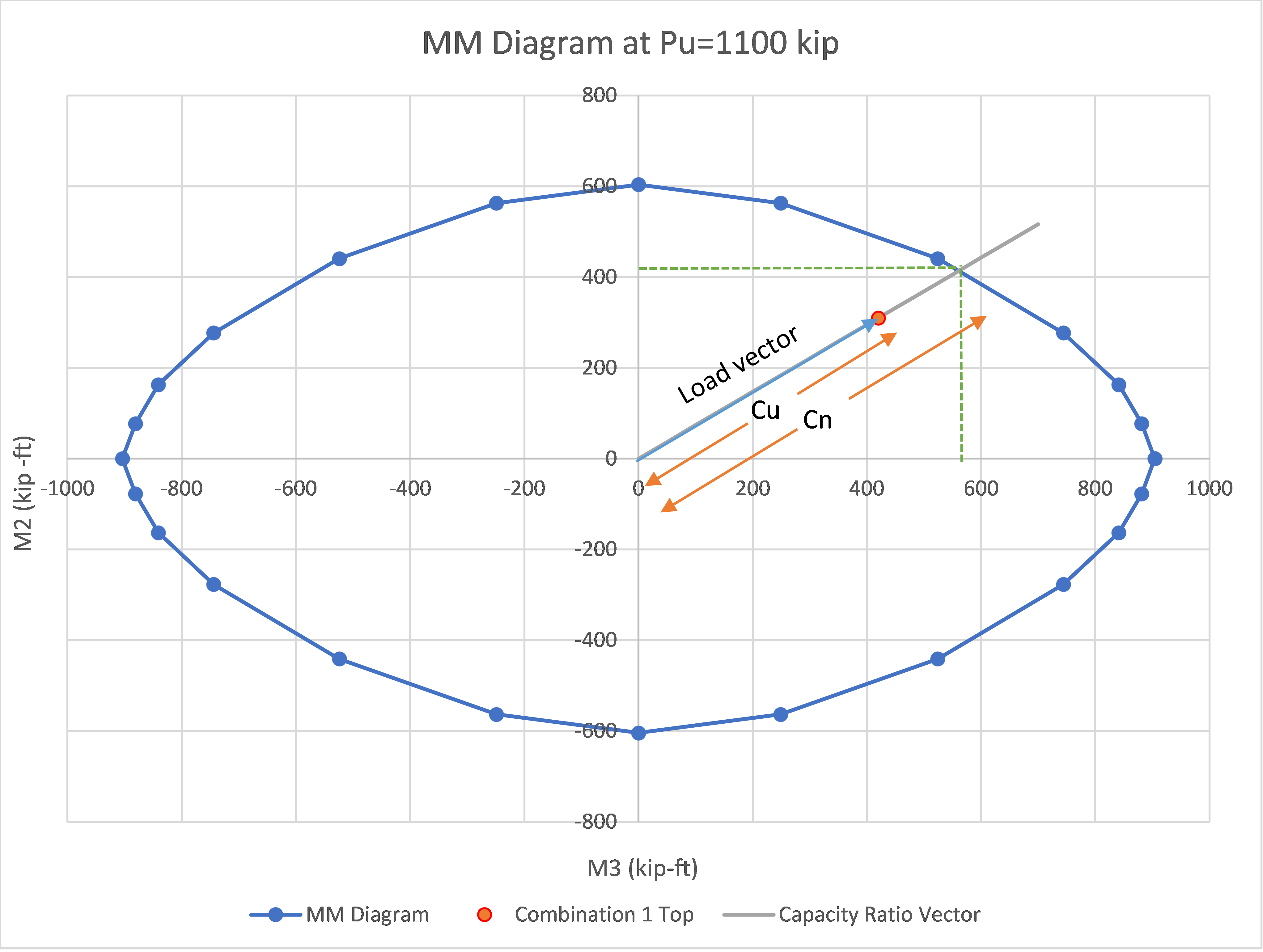
Figure 1 : MM Curve for Combination 1
Combination 2 (Top End)
Moment Sum at P
Moment sum D/C = \(\frac{M_{2u}}{{Ф\ M}_{2n,max}}\ + \ \frac{M_{3u}}{{Ф\ M}_{3n,max}}\) = \(\frac{65}{227}\ + \ \frac{110}{338}\) = \(0.61\)
Moment Vector at P
\(C_{u} = \ \sqrt{M_{2u}^{2} + M_{3u}^{2}}\) = \(\sqrt{65^{2} + \ 110^{2}\ }\)=\(\ 127.77\ kip - ft\)
\(C_{n} = \ \sqrt{M_{2n}^{2} + M_{3n}^{2}}\) = \(\sqrt{177^{2} + \ 303^{2}\ }\)=\(\ 350.91\ kip - ft\)
Moment Vector D/C = \(\frac{C_{u}}{C_{n}}\) = \(\frac{127.77}{350.91} = \ 0.36\)
Axial Compression Capacity
Axial Compression D/C = \(0.00\)
Axial Tension Capacity
Axial Tension D/C = \(\frac{P_{u}}{{Ф\ P}_{n,\max}}\) \(= \frac{60}{313} = \ 0.19\)
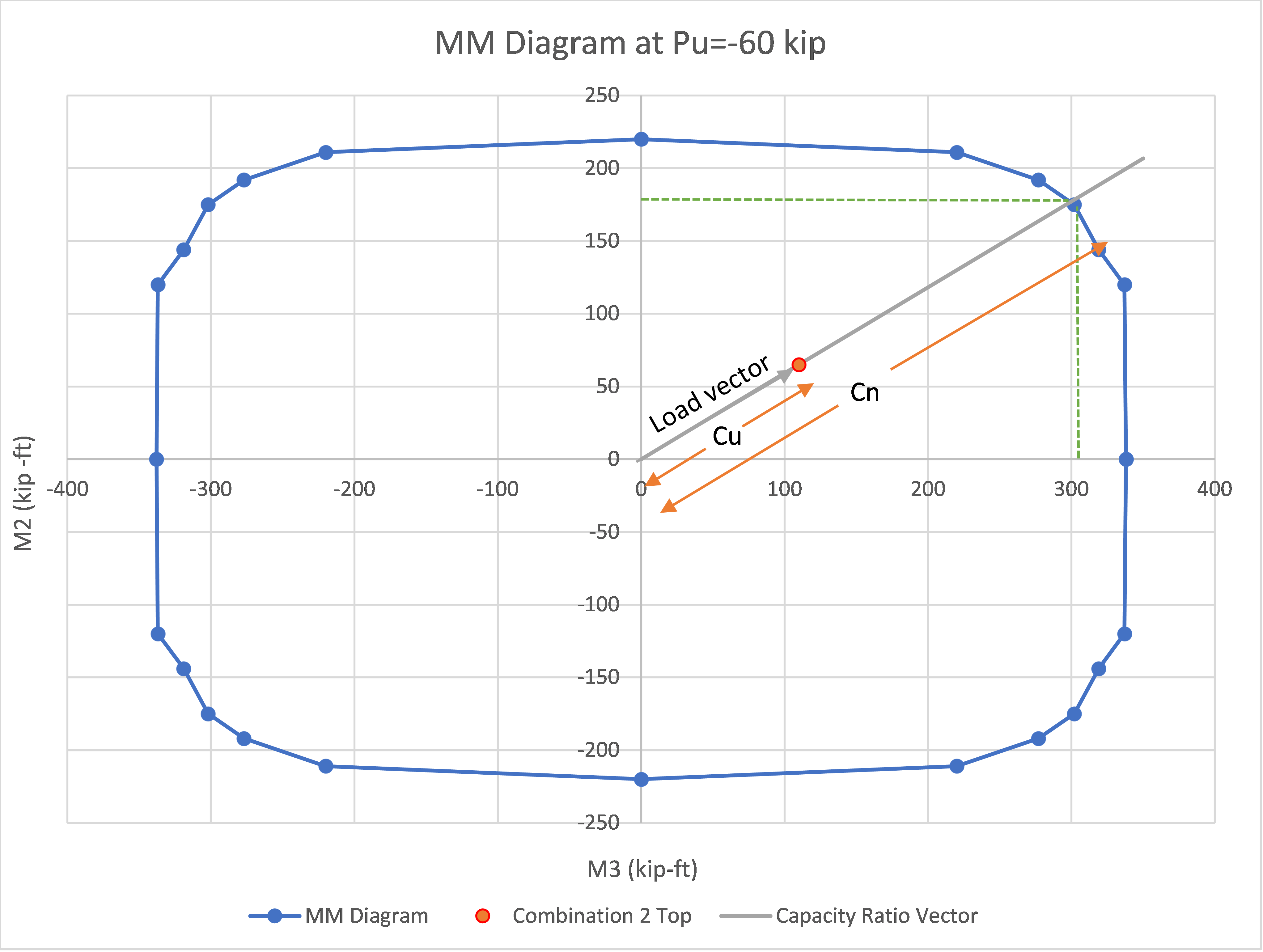
Figure 2 : MM Curve for Combination 2
DC - Example 002
Capacity Ratio Check for Circular Column
GEOMETRY, PROPERTIES AND LOADING
The Capacity Ratio Check for a given circular section is tested in this example by comparing the results with hand calculations.
The column section details and loading details are as tabulated below.
Note: Refer DC Ex002.cdbx
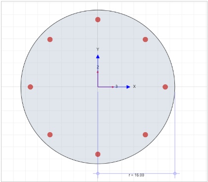
| Parameters | Column Designer |
|---|---|
| Radius (in) | 16 |
| fc’ (psi) | 4,000 |
| fy (psi) | 40,000 |
| Rebar | #8 |
| Number of bars | 8 |
| Rebar Area (in2) | 6.28 |
| Rebar Ratio | 0.78% |
| Clear Cover (in) | 1.5 |
| Name | Axial Load, Pu (kip) | Moment Top, Mux (kip-ft) | Moment Top, Muy (kip-ft) | Moment Bottom, Mux (kip-ft) | Moment Bottom, Muy (kip-ft) |
|---|---|---|---|---|---|
| Combination 1 | 1200 | 300 | 105 | 200 | 105 |
| Combination 2 | -70 | -100 | 60 | -75 | 55 |
CAPACITY RATIO COMPARISON
Column Designer reports 4 types of capacity ratios namely: Moment sum at P, Moment Vector at P, Axial Compression Capacity and Axial Tension Capacity. The values obtained are tabulated below followed by the detailed hand calculation.
Combination 1 (Top End)
| Capacity Ratios | Column Designer | By hand |
|---|---|---|
| Moment sum at P | 0.75 | 0.75 |
| Moment Vector at P | 0.59 | 0.59 |
| Axial Compression Capacity | 0.77 | 0.77 |
| Axial Tension Capacity | 0.00 | 0.00 |
Combination 2 (Top End)
| Capacity Ratios | Column Designer | By hand |
|---|---|---|
| Moment sum at P | 0.88 | 0.88 |
| Moment Vector at P | 0.65 | 0.65 |
| Axial Compression Capacity | 0.00 | 0.00 |
| Axial Tension Capacity | 0.31 | 0.31 |
CALCULATIONS BY HAND
Combination 1 (Top End)
Moment Sum at P
Moment sum D/C = \(\frac{M_{2u}}{{Ф\ M}_{2n,max}}\ + \ \frac{M_{3u}}{{Ф\ M}_{3n,max}}\) = \(\frac{105}{537}\ + \ \frac{300}{537}\) = \(0.75\\)
Moment Vector at P
\(C_{u} = \ \sqrt{M_{2u}^{2} + M_{3u}^{2}}\) = \(\sqrt{105^{2} + \ 300^{2}\ }\)=\(\ 317.84\ kip - ft\)
\(C_{n} = \ \sqrt{M_{2n}^{2} + M_{3n}^{2}}\) = \(\sqrt{165^{2} + \ 515^{2}\ }\)=\(\ 540.79\ kip - ft\)
Moment Vector D/C = \(\frac{C_{u}}{C_{n}}\) = \(\frac{317.84}{540.79} = \ 0.59\)
Axial Compression Capacity
Axial Compression D/C = \(\frac{P_{u}}{{Ф\ P}_{n,max}}\) \(= \frac{1,200}{1,550} = \ 0.77\)
Axial Tension Capacity
Axial Tension D/C = \(0.00\)
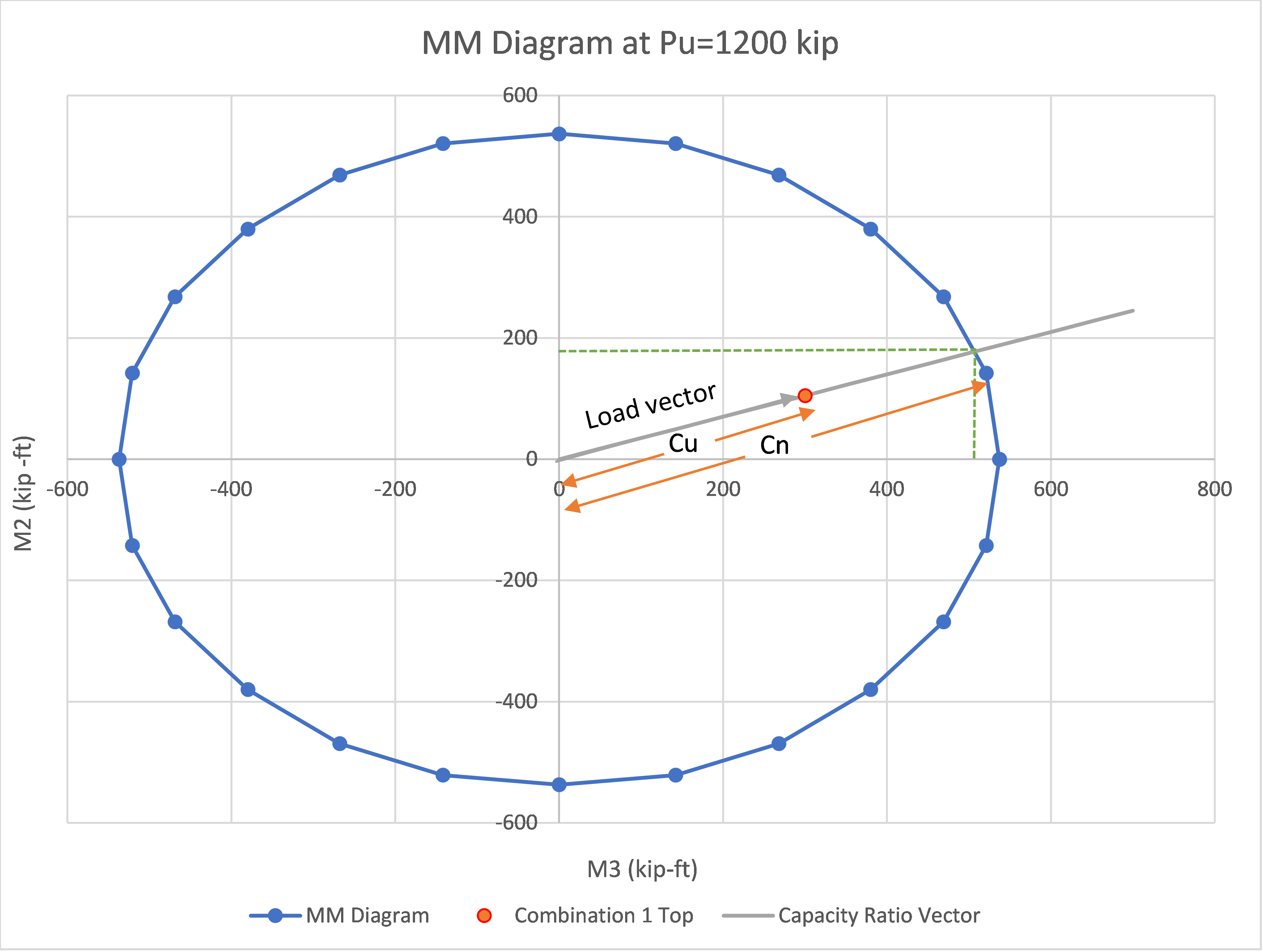
Figure 3 : MM Curve for Combination 1
Combination 2 (Top End)
Moment Sum at P
Moment sum D/C = \(\frac{M_{2u}}{{Ф\ M}_{2n,max}}\ + \ \frac{M_{3u}}{{Ф\ M}_{3n,max}}\) = \(\frac{60}{181.4}\ + \ \frac{100}{181.4}\) = \(0.88\)
Moment Vector at P
\(C_{u} = \ \sqrt{M_{2u}^{2} + M_{3u}^{2}}\) = \(\sqrt{60^{2} + \ 100^{2}\ }\)=\(\ 116.62\ kip - ft\)
\(C_{n} = \ \sqrt{M_{2n}^{2} + M_{3n}^{2}}\) = \(\sqrt{92^{2} + \ 153^{2}\ }\)=\(\ 178.53\ kip - ft\)
Moment Vector D/C = \(\frac{C_{u}}{C_{n}}\) = \(\frac{116.62}{178.53} = \ 0.65\)
Axial Compression Capacity
Axial Compression D/C = \(0.00\)
Axial Tension Capacity
Axial Tension D/C = \(\frac{P_{u}}{{Ф\ P}_{n,max}}\) \(= \frac{70}{226.19} = \ 0.31\)
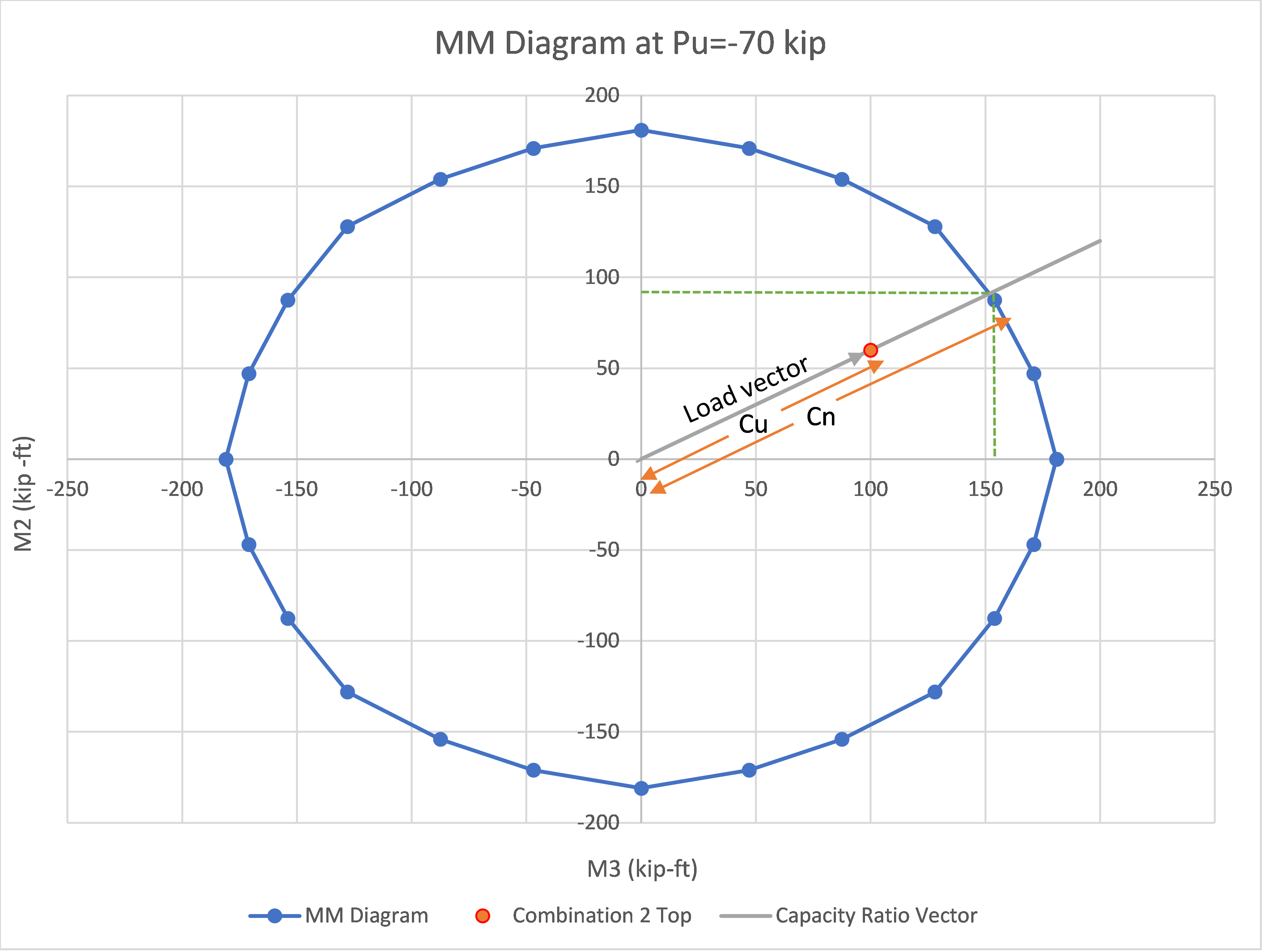
Figure 4 : MM Curve for Combination 2
DC - Example 003
Capacity Ratio Check for T-Section
GEOMETRY, PROPERTIES AND LOADING
The Capacity Ratio Check for a given T-section section is tested in this example by comparing the results with hand calculations.
Note: Refer DC Ex003.cdbx
The column section details and loading details are as tabulated below.
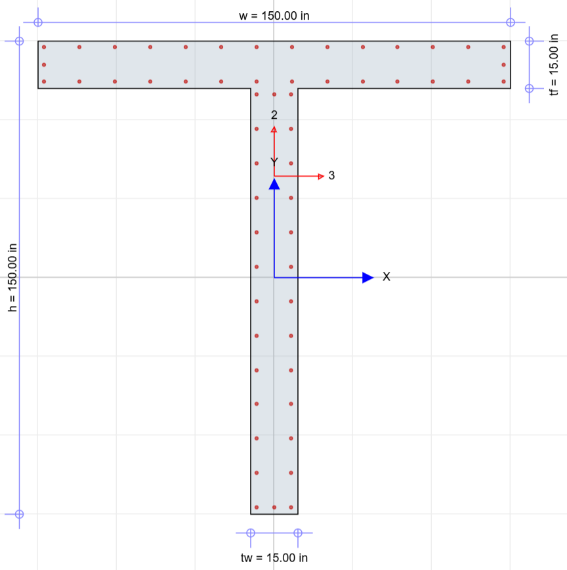
| Parameters | Column Designer |
|---|---|
| Height (in) | 150 |
| Width (in) | 150 |
| Web Width (in) | 15 |
| Flange Height (in) | 15 |
| fc’ (psi) | 6,000 |
| fy (psi) | 60,000 |
| Number of bars | 58 |
| Corner Bars | #8 |
| Bars along direction 2 and 3 | #8 |
| Rebar Area (in2) | 45.55 |
| Rebar Ratio | 1.07% |
| Clear Cover (in) | 1.5 |
| Name | Axial Load, Pu (kip) | Moment Top, Mux (kip-ft) | Moment Top, Muy (kip-ft) | Moment Bottom, Mux (kip-ft) | Moment Bottom, Muy (kip-ft) |
|---|---|---|---|---|---|
| Combination 1 | 10,000 | 0 | 0 | 15,000 | 0 |
| Combination 2 | 10,000 | 0 | 0 | -15,000 | 0 |
CAPACITY RATIO COMPARISON
Column Designer reports 4 types of capacity ratios namely: Moment sum at P, Moment Vector at P, Axial Compression Capacity and Axial Tension Capacity. The values obtained are tabulated below followed by the detailed hand calculation.
Combination 1 (Bottom End)
| Capacity Ratios | Column Designer | By hand |
|---|---|---|
| Moment sum at P | 0.40 | 0.40 |
| Moment Vector at P | 0.40 | 0.40 |
| Axial Compression Capacity | 0.79 | 0.79 |
| Axial Tension Capacity | 0.00 | 0.00 |
| Capacity Ratios | Column Designer | By hand |
|---|---|---|
| Moment sum at P | 0.85 | 0.85 |
| Moment Vector at P | 0.85 | 0.85 |
| Axial Compression Capacity | 0.79 | 0.79 |
| Axial Tension Capacity | 0.00 | 0.00 |
Combination 2 (Bottom End)
CALCULATIONS BY HAND
Combination 1 (Bottom End)
Moment Sum at P
Moment sum D/C = \(\frac{M_{2u}}{{Ф\ M}_{2n,max}}\ + \ \frac{M_{3u}}{{Ф\ M}_{3n,max}}\) = \(\frac{0}{14,181}\ + \ \frac{15,000}{37,086}\) = \(0.40\\)
Moment Vector at P
\(C_{u} = \ \sqrt{M_{2u}^{2} + M_{3u}^{2}}\) = \(\sqrt{0^{2} + \ {15,000}^{2}\ }\)=\(\ 15,000\ kip - ft\)
\(C_{n} = \ \sqrt{M_{2n}^{2} + M_{3n}^{2}}\) = \(\sqrt{0^{2} + \ {37,086}^{2}\ }\)=\(\ 37,086\ kip - ft\)
Moment Vector D/C = \(\frac{C_{u}}{C_{n}}\) = \(\frac{15,000}{37,086} = \ 0.40\)
Axial Compression Capacity
Axial Compression D/C = \(\frac{P_{u}}{{Ф\ P}_{n,max}}\) \(= \frac{10,000}{12,645} = \ 0.79\)
Axial Tension Capacity
Axial Tension D/C = \(0.00\)
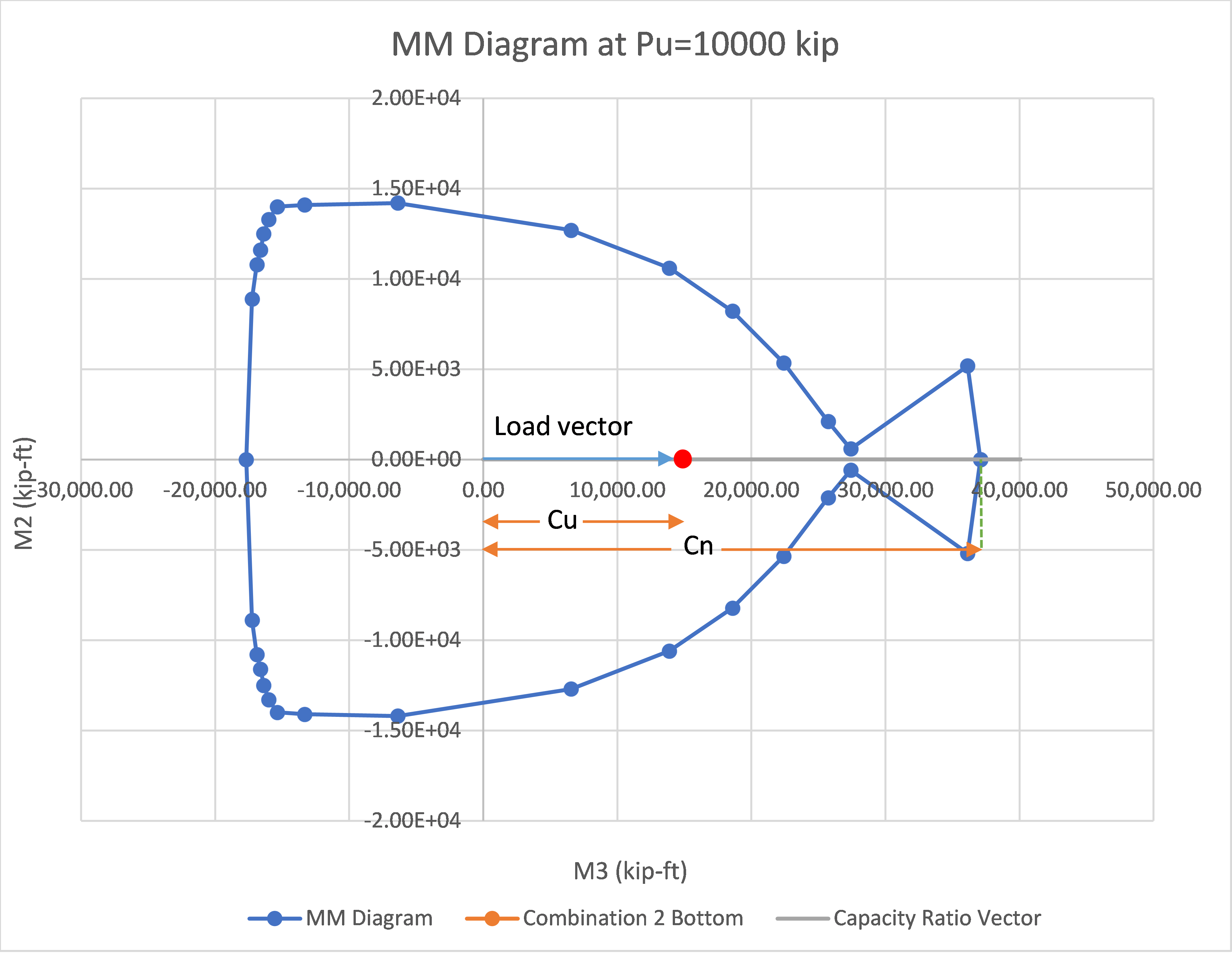
Figure 5 : MM Curve for Combination 1
Combination 2 (Bottom End)
Moment Sum at P
Moment sum D/C = \(\frac{M_{2u}}{{Ф\ M}_{2n,max}}\ + \ \frac{M_{3u}}{{Ф\ M}_{3n,max}}\) = \(\frac{0}{14,181}\ + \ \frac{- 15,000}{- 17,682}\) = \(0.85\)
Moment Vector at P
\(C_{u} = \ \sqrt{M_{2u}^{2} + M_{3u}^{2}}\) = \(\sqrt{0^{2} + \ {- 15,000}^{2}\ }\)=\(\ 15,000\ kip - ft\)
\(C_{n} = \ \sqrt{M_{2n}^{2} + M_{3n}^{2}}\) = \(\sqrt{0^{2} + \ {- 17,682}^{2}\ }\)=\(\ 17,682\ kip - ft\)
Moment Vector D/C = \(\frac{C_{u}}{C_{n}}\) = \(\frac{15,000}{17,682} = \ 0.85\)
Axial Compression Capacity
Axial Compression D/C = \(\frac{P_{u}}{{Ф\ P}_{n,max}}\) \(= \frac{10,000}{12,645} = \ 0.79\)
Axial Tension Capacity
Axial Tension D/C = \(0.00\)
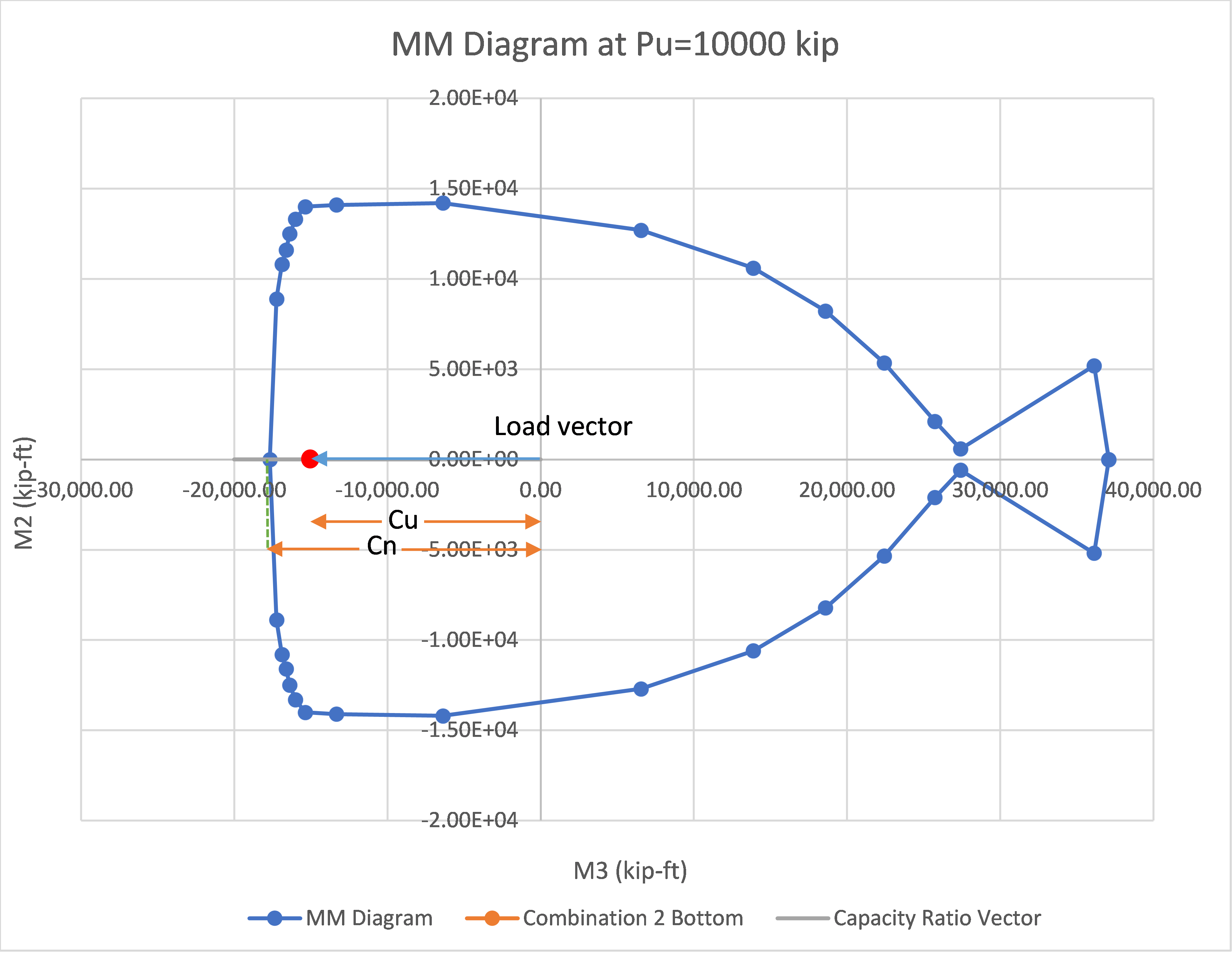
Figure 6 : MM Curve for Combination 2
DC - Example 004
Capacity Ratio Check for T-Section
GEOMETRY, PROPERTIES AND LOADING
The Capacity Ratio Check for a given T-section section is tested in this example by comparing the results with hand calculations.
Note: Refer DC Ex004.cdbx
The column section details and loading details are as tabulated below.
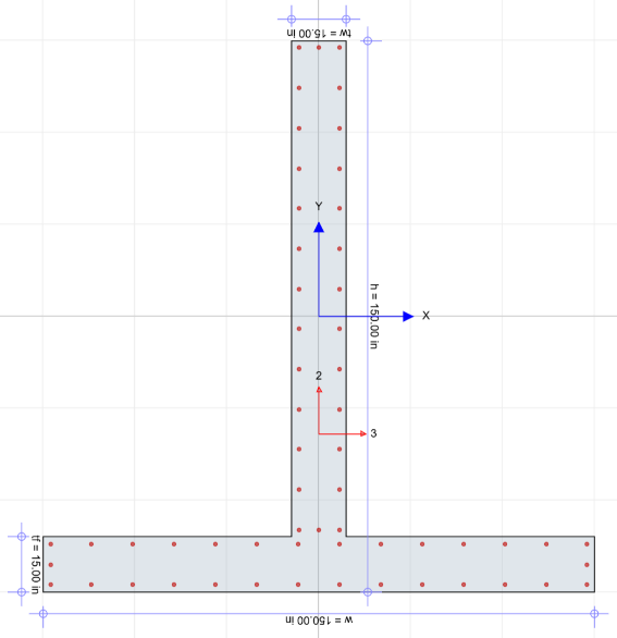
| Parameters | Column Designer |
|---|---|
| Height (in) | 150 |
| Width (in) | 150 |
| Web Width (in) | 15 |
| Flange Height (in) | 15 |
| fc’ (psi) | 6,000 |
| fy (psi) | 60,000 |
| Number of bars | 58 |
| Corner Bars | #8 |
| Bars along direction 2 and 3 | #8 |
| Rebar Area (in2) | 45.55 |
| Rebar Ratio | 1.07% |
| Clear Cover (in) | 1.5 |
| Name | Axial Load, Pu (kip) | Moment Top, Mux (kip-ft) | Moment Top, Muy (kip-ft) | Moment Bottom, Mux (kip-ft) | Moment Bottom, Muy (kip-ft) |
|---|---|---|---|---|---|
| Combination 1 | 10,000 | 0 | 0 | 15,000 | 0 |
| Combination 2 | 10,000 | 0 | 0 | -15,000 | 0 |
CAPACITY RATIO COMPARISON
Column Designer reports 4 types of capacity ratios namely: Moment sum at P, Moment Vector at P, Axial Compression Capacity and Axial Tension Capacity. The values obtained are tabulated below followed by the detailed hand calculation.
Combination 1 (Bottom End)
| Capacity Ratios | Column Designer | By hand |
|---|---|---|
| Moment sum at P | 0.85 | 0.85 |
| Moment Vector at P | 0.85 | 0.85 |
| Axial Compression Capacity | 0.79 | 0.79 |
| Axial Tension Capacity | 0.00 | 0.00 |
| Capacity Ratios | Column Designer | By hand |
|---|---|---|
| Moment sum at P | 0.40 | 0.40 |
| Moment Vector at P | 0.40 | 0.40 |
| Axial Compression Capacity | 0.79 | 0.79 |
| Axial Tension Capacity | 0.00 | 0.00 |
Combination 2 (Bottom End)
CALCULATIONS BY HAND
Combination 1 (Bottom End)
Moment Sum at P
Moment sum D/C = \(\frac{M_{2u}}{{Ф\ M}_{2n,max}}\ + \ \frac{M_{3u}}{{Ф\ M}_{3n,max}}\) = \(\frac{0}{14,181}\ + \ \frac{15,000}{17,682}\) = \(0.85\)
Moment Vector at P
\(C_{u} = \ \sqrt{M_{2u}^{2} + M_{3u}^{2}}\) = \(\sqrt{0^{2} + \ {15,000}^{2}\ }\)=\(\ 15,000\ kip - ft\)
\(C_{n} = \ \sqrt{M_{2n}^{2} + M_{3n}^{2}}\) = \(\sqrt{0^{2} + \ {17,682}^{2}\ }\)=\(\ 17,682\ kip - ft\)
Moment Vector D/C = \(\frac{C_{u}}{C_{n}}\) = \(\frac{15,000}{17,682} = \ 0.85\)
Axial Compression Capacity
Axial Compression D/C = \(\frac{P_{u}}{{Ф\ P}_{n,max}}\) \(= \frac{10,000}{12,645} = \ 0.79\)
Axial Tension Capacity
Axial Tension D/C = \(0.00\)
Figure 7 : MM Curve for Combination 1
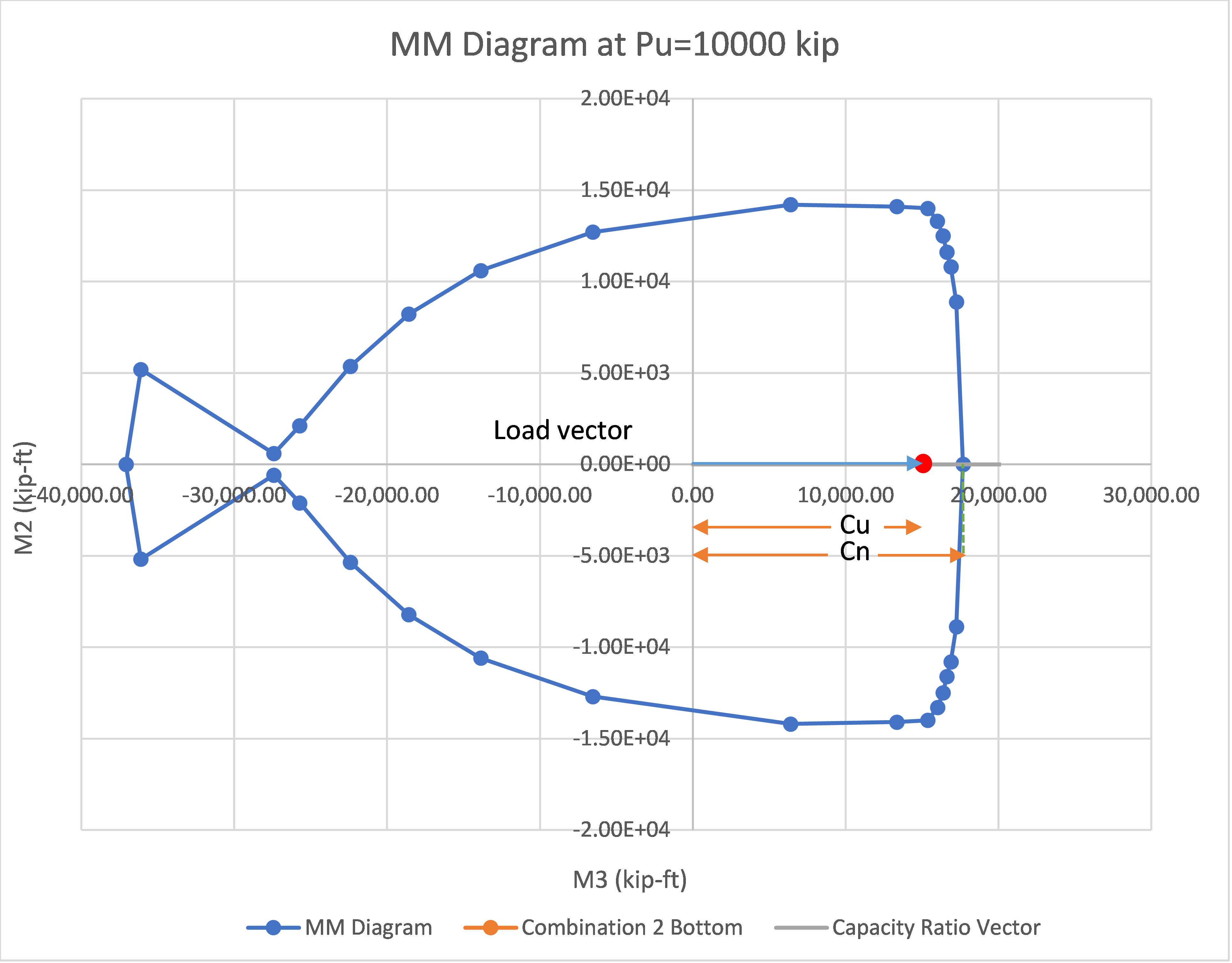
Combination 1 (Bottom End)
Moment Sum at P
Moment sum D/C = \(\frac{M_{2u}}{{Ф\ M}_{2n,max}}\ + \ \frac{M_{3u}}{{Ф\ M}_{3n,max}}\) = \(\frac{0}{14,181}\ + \ \frac{- 15,000}{- 37,086}\) = \(0.40\\)
Moment Vector at P
\(C_{u} = \ \sqrt{M_{2u}^{2} + M_{3u}^{2}}\) = \(\sqrt{0^{2} + \ {- 15,000}^{2}\ }\)=\(\ 15,000\ kip - ft\)
\(C_{n} = \ \sqrt{M_{2n}^{2} + M_{3n}^{2}}\) = \(\sqrt{0^{2} + \ {- 37,086}^{2}\ }\)=\(\ 37,086\ kip - ft\)
Moment Vector D/C = \(\frac{C_{u}}{C_{n}}\) = \(\frac{15,000}{37,086} = \ 0.40\)
Axial Compression Capacity
Axial Compression D/C = \(\frac{P_{u}}{{Ф\ P}_{n,max}}\) \(= \frac{10,000}{12,645} = \ 0.79\)
Axial Tension Capacity
Axial Tension D/C = \(0.00\)
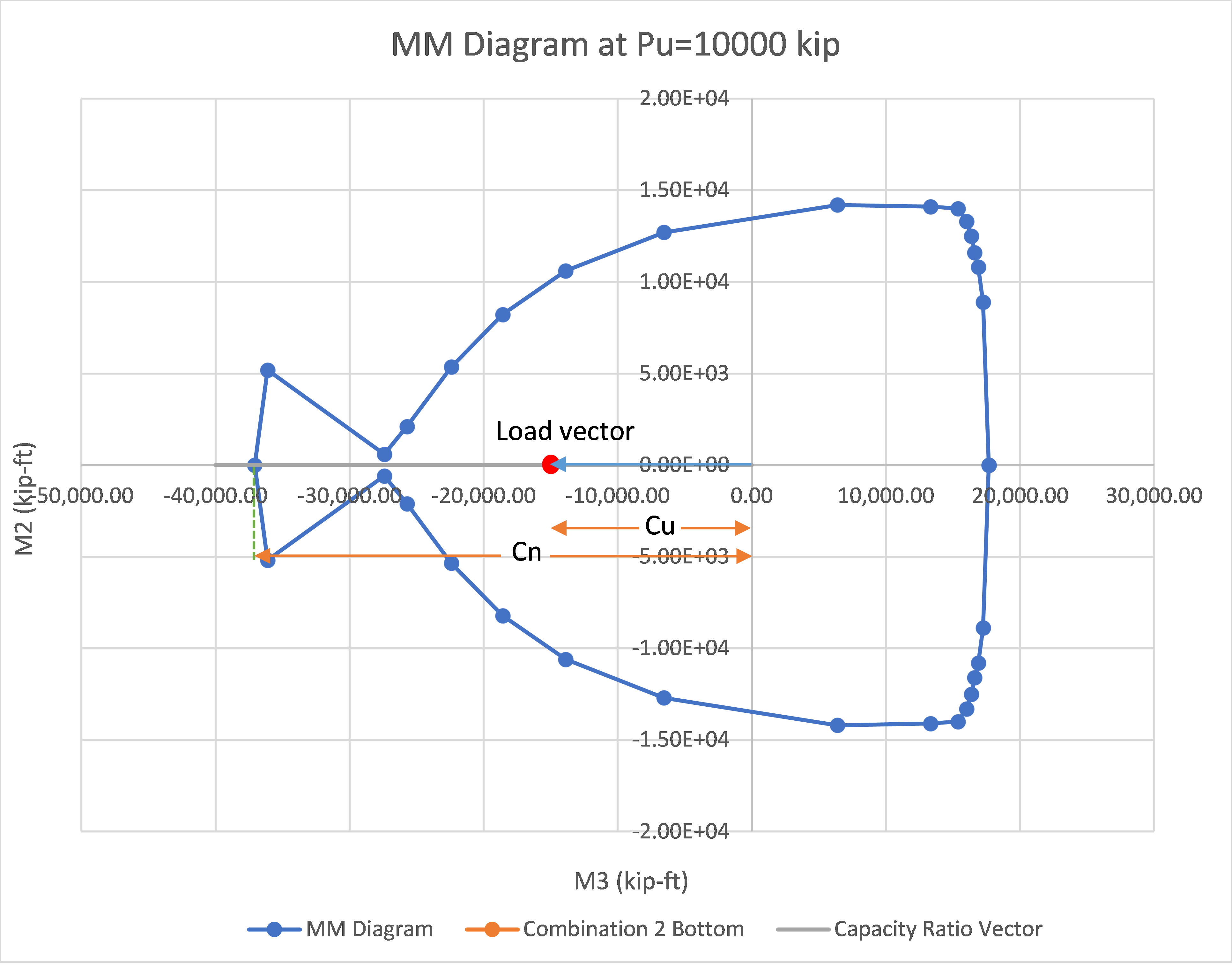
Figure 2 : MM Curve for Combination 2
Moment Curvature
Moment Curvature Example 001
Moment Curvature Check for Rectangular Column
GEOMETRY AND PROPERTIES
The Moment Curvature for a given rectangular section is tested in this example by comparing the results with SAP2000 v26.
Note: Refer Moment Curvature Ex001.cdbx
The column section details are as tabulated below.
| Parameters | Column Designer | SAP2000 v26 |
|---|---|---|
| Code | ACI 318-19 | |
| Height (in) | 36 | |
| Width (in) | 24 | |
| fc’ (psi) | 4,000 | |
| fy (psi) | 40,000 | |
| Number of bars | 10 | |
| Corner Bars | #9 | |
| Bars along direction 2 and 3 | #8 | |
| Rebar Area (in2) | 8.71 | |
| Rebar Ratio | 1.01% | |
| Clear Cover (in) | 1.5 | |
CONCRETE MATERIAL PROPERTIES
| Parameters | Value |
| Concrete Material Properties | |
| Specified Concrete Compressive Strength, fc’ (psi) | 4,000 |
| Modulus of Elasticity, E (psi) | 3,605,000 |
| Concrete Stress Strain Model Properties | |
| Stress Strain Model | Mander’s Unconfined |
| Strain at Unconfined Compressive Strength (fc’) | 0.002 |
| Ultimate Unconfined Strain Capacity | 0.005 |
REBAR MATERIAL PROPERTIES
| Parameters | Value |
| Rebar Material Properties | |
| Minimum Yield Stress, fy (psi) | 40,000 |
| Minimum Tensile Stress, fu (psi) | 60,000 |
| Modulus of Elasticity, E (psi) | 29,000,000 |
| Rebar Stress Strain Model Properties | |
| Stress Strain Model | Park Strain Hardening |
| Strain at Onset of Strain Hardening (εsh) | 0.02 |
| Ultimate Strain Capacity (εsu) | 0.12 |
MOMENT CURVATURE DIAGRAM PROPERTIES
| Parameters | Value |
| Angle | 0 |
| Maximum Compression Strain (10-3 in/in) | 100 |
| Maximum Tension Strain (10-3 in/in) | 500 |
| Maximum Curvature (10-3 rad/in) | 100 |
MOMENT CURVATURE COMPARISON WITH AXIAL LOAD (P) = 0 Kips
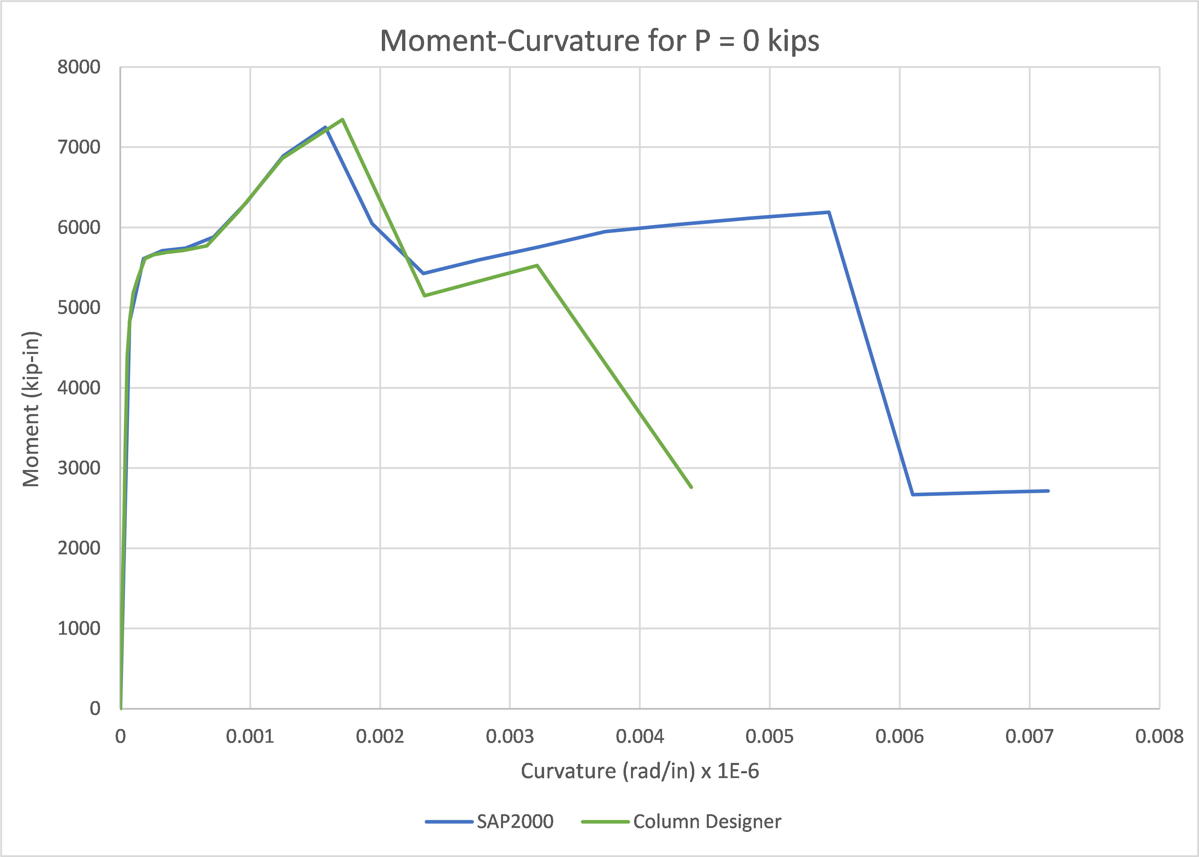
Moment Curvature Example 002
Moment Curvature Check for Rectangular Column
GEOMETRY AND PROPERTIES
The Moment Curvature for a given rectangular section is tested in this example by comparing the results with SAP2000 v26.
Note: Refer Moment Curvature Ex002.cdbx
The column section details are as tabulated below.
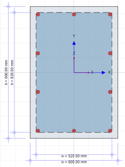
| Parameters | Column Designer | SAP2000 v26 |
|---|---|---|
| Code | ACI 318-19 | |
| Height (mm) | 900 | |
| Width (mm) | 600 | |
| fc’ (MPa) | 27.58 | |
| fy (MPa) | 413.69 | |
| Number of bars | 10 | |
| Corner Bars | d 25 | |
| Bars along direction 2 and 3 | d 25 | |
| Rebar Area (mm2) | 4908.74 | |
| Rebar Ratio | 0.91% | |
| Clear Cover (mm) | 40 | |
CONCRETE MATERIAL PROPERTIES
| Parameters | Value |
| Concrete Material Properties | |
| Specified Concrete Compressive Strength, fc’ (MPa) | 27.58 |
| Modulus of Elasticity, E (MPa) | 24855.58 |
| Ultimate Strain Capacity (Unconfined) | 0.005 |
| Concrete Stress Strain Model Properties | |
| Stress Strain Model | Mander’s Confined |
| Strain at Compressive Strength (fc’) | 0.00219 |
| Maximum Strain | 0.05 |
| Width of confinement zone (mm) | 520 |
| Height of confinement zone (mm) | 820 |
| Tie Bar Strength, fy (MPa) | 413.69 |
| Tie Spacing Along X (mm) | 545 |
| Tie Diameter Along X (mm) | 25 |
| Tie Spacing Along Y (mm) | 845 |
| Tie Diameter Along Y (mm) | 25 |
| Vertical Spacing of Ties (mm) | 250 |
| Total Main Steel (mm2) | 4908.74 |
REBAR MATERIAL PROPERTIES
| Parameters | Value |
| Rebar Material Properties | |
| Minimum Yield Stress, fy (MPa) | 413.69 |
| Minimum Tensile Stress, fu (MPa) | 620.53 |
| Modulus of Elasticity, E (MPa) | 199948.04 |
| Rebar Stress Strain Model Properties | |
| Stress Strain Model | Park Strain Hardening |
| Strain at Onset of Strain Hardening (εsh) | 0.01 |
| Ultimate Strain Capacity (εsu) | 0.09 |
MOMENT CURVATURE DIAGRAM PROPERTIES
| Parameters | Value |
| Angle | 0 |
| Maximum Compression Strain (10-3 mm/mm) | 100 |
| Maximum Tension Strain (10-3 mm/mm) | 500 |
| Maximum Curvature (10-3 rad/mm) | 4 |
MOMENT CURVATURE COMPARISON WITH AXIAL LOAD (P) = 0 kN